Function File: specgram (x) ¶

Function File: specgram (x, n) ¶

Function File: specgram (x, n, Fs) ¶

Function File: specgram (x, n, Fs, window) ¶

Function File: specgram (x, n, Fs, window, overlap) ¶

Function File: [S, f, t] = specgram (…) ¶

Generate a spectrogram for the signal x. The signal is chopped into overlapping segments of length n, and each segment is windowed and transformed into the frequency domain using the FFT. The default segment size is 256. If fs is given, it specifies the sampling rate of the input signal. The argument window specifies an alternate window to apply rather than the default of hanning (n). The argument overlap specifies the number of samples overlap between successive segments of the input signal. The default overlap is length (window)/2.

If no output arguments are given, the spectrogram is displayed. Otherwise, S is the complex output of the FFT, one row per slice, f is the frequency indices corresponding to the rows of S, and t is the time indices corresponding to the columns of S.

Example:

   x = chirp([0:0.001:2],0,2,500);  # freq. sweep from 0-500 over 2 sec.
   Fs=1000;                  # sampled every 0.001 sec so rate is 1 kHz
   step=ceil(20*Fs/1000);    # one spectral slice every 20 ms
   window=ceil(100*Fs/1000); # 100 ms data window
   specgram(x, 2^nextpow2(window), Fs, window, window-step);

   ## Speech spectrogram
   [x, Fs] = auload(file_in_loadpath("sample.wav")); # audio file
   step = fix(5*Fs/1000);     # one spectral slice every 5 ms
   window = fix(40*Fs/1000);  # 40 ms data window
   fftn = 2^nextpow2(window); # next highest power of 2
   [S, f, t] = specgram(x, fftn, Fs, window, window-step);
   S = abs(S(2:fftn*4000/Fs,:)); # magnitude in range 0<f<=4000 Hz.
   S = S/max(S(:));           # normalize magnitude so that max is 0 dB.
   S = max(S, 10^(-40/10));   # clip below -40 dB.
   S = min(S, 10^(-3/10));    # clip above -3 dB.
   imagesc (t, f, log(S));    # display in log scale
   set (gca, "ydir", "normal"); # put the 'y' direction in the correct direction

The choice of window defines the time-frequency resolution. In speech for example, a wide window shows more harmonic detail while a narrow window averages over the harmonic detail and shows more formant structure. The shape of the window is not so critical so long as it goes gradually to zero on the ends.

Step size (which is window length minus overlap) controls the horizontal scale of the spectrogram. Decrease it to stretch, or increase it to compress. Increasing step size will reduce time resolution, but decreasing it will not improve it much beyond the limits imposed by the window size (you do gain a little bit, depending on the shape of your window, as the peak of the window slides over peaks in the signal energy). The range 1-5 msec is good for speech.

FFT length controls the vertical scale. Selecting an FFT length greater than the window length does not add any information to the spectrum, but it is a good way to interpolate between frequency points which can make for prettier spectrograms.

After you have generated the spectral slices, there are a number of decisions for displaying them. First the phase information is discarded and the energy normalized:

S = abs(S); S = S/max(S(:));

Then the dynamic range of the signal is chosen. Since information in speech is well above the noise floor, it makes sense to eliminate any dynamic range at the bottom end. This is done by taking the max of the magnitude and some minimum energy such as minE=-40dB. Similarly, there is not much information in the very top of the range, so clipping to a maximum energy such as maxE=-3dB makes sense:

S = max(S, 10^(minE/10)); S = min(S, 10^(maxE/10));

The frequency range of the FFT is from 0 to the Nyquist frequency of one half the sampling rate. If the signal of interest is band limited, you do not need to display the entire frequency range. In speech for example, most of the signal is below 4 kHz, so there is no reason to display up to the Nyquist frequency of 10 kHz for a 20 kHz sampling rate. In this case you will want to keep only the first 40% of the rows of the returned S and f. More generally, to display the frequency range [minF, maxF], you could use the following row index:

idx = (f >= minF & f <= maxF);

Then there is the choice of colormap. A brightness varying colormap such as copper or bone gives good shape to the ridges and valleys. A hue varying colormap such as jet or hsv gives an indication of the steepness of the slopes. The final spectrogram is displayed in log energy scale and by convention has low frequencies on the bottom of the image:

imagesc(t, f, flipud(log(S(idx,:))));

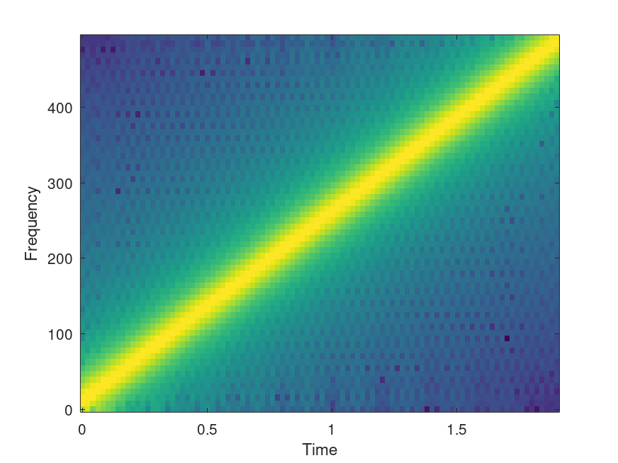
Demonstration 1

Package: signal