- Function File:
[w, xmu] =ultrwin(m, mu, beta)¶ - Function File:
[w, xmu] =ultrwin(m, mu, att, "att")¶ - Function File:
[w, xmu] =ultrwin(m, mu, latt, "latt")¶ - Function File:
w =ultrwin(m, mu, xmu, "xmu")¶ Return the coefficients of an Ultraspherical window of length m. The parameter mu controls the window’s Fourier transform’s side-lobe to side-lobe ratio, and the third given parameter controls the transform’s main-lobe width/side-lobe-ratio; normalize w such that the central coefficient(s) value is unitary.
By default, the third parameter is beta, which sets the main lobe width to beta times that of a rectangular window. Alternatively, giving att or latt sets the ripple ratio at the first or last side-lobe respectively, or giving xmu sets the (un-normalized) window’s Fourier transform according to its canonical definition:
             (MU)
     W(k) = C   [ XMU cos(pi k/M) ],  k = 0, 1, ..., M-1,
             M-1
where C is the Ultraspherical (a.k.a. Gegenbauer) polynomial, which can be defined using the recurrence relationship:
      (l)    1                  (l)                    (l)
     C (x) = - [ 2x(m + l - 1) C   (x) - (m + 2l - 2) C   (x) ]
      m      m                  m-1                    m-2

                                (l)        (l)
     for m an integer > 1, and C (x) = 1, C (x) = 2lx.
                                0          1
For given beta, att, or latt, the corresponding (determined) value of xmu is also returned.
The Dolph-Chebyshev and Saramaki windows are special cases of the Ultraspherical window, with mu set to 0 and 1 respectively. Note that when not giving xmu, stability issues may occur with mu <= -1.5. For further information about the window, see
- Kabal, P., 2009: Time Windows for Linear Prediction of Speech. Technical Report, Dept. Elec. & Comp. Eng., McGill University.
- Bergen, S., Antoniou, A., 2004: Design of Ultraspherical Window Functions with Prescribed Spectral Characteristics. Proc. JASP, 13/13, pp. 2053-2065.
- Streit, R., 1984: A two-parameter family of weights for nonrecursive digital filters and antennas. Trans. ASSP, 32, pp. 108-118.
See also: chebwin, kaiser.
Demonstration 1
The following code
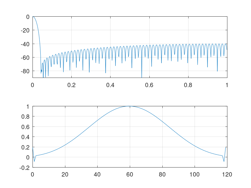
 w=ultrwin(120, -1, 40, "l"); [W,f]=freqz(w); clf
 subplot(2,1,1); plot(f/pi, 20*log10(W/abs(W(1)))); grid; axis([0 1 -90 0])
 subplot(2,1,2); plot(0:length(w)-1, w); grid
 %-----------------------------------------------------------
 % Figure shows an Ultraspherical window with MU=-1, LATT=40:
 % frequency domain above, time domain below.
Produces the following figure
| Figure 1 |
|---|
 |
Demonstration 2
The following code
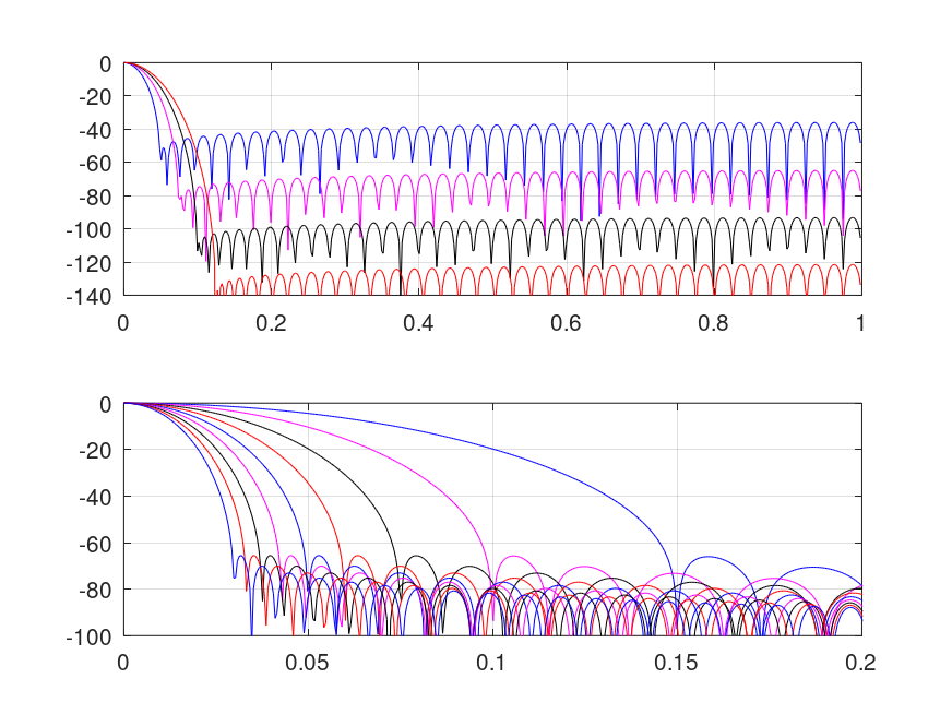
 c="krbm"; clf; subplot(2, 1, 1)
 for beta=2:5
   w=ultrwin(80, -.5, beta); [W,f]=freqz(w);
   plot(f/pi, 20*log10(W/abs(W(1))), c(1+mod(beta, length(c)))); hold on
 end; grid; axis([0 1 -140 0]); hold off
 subplot(2, 1, 2);
 for n=2:10
   w=ultrwin(n*20, 1, 3); [W,f]=freqz(w,1,2^11);
   plot(f/pi, 20*log10(W/abs(W(1))), c(1+mod(n, length(c)))); hold on
 end; grid; axis([0 .2 -100 0]); hold off
 %--------------------------------------------------
 % Figure shows transfers of Ultraspherical windows:
 % above: varying BETA with fixed N & MU,
 % below: varying N with fixed MU & BETA.
Produces the following figure
| Figure 1 |
|---|
 |
Demonstration 3
The following code
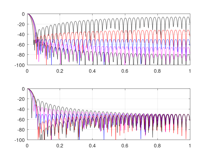
 c="krbm"; clf; subplot(2, 1, 1)
 for j=0:4
   w=ultrwin(80, j*.6-1.2, 50, "a"); [W,f]=freqz(w);
   plot(f/pi, 20*log10(W/abs(W(1))), c(1+mod(j, length(c)))); hold on
 end; grid; axis([0 1 -100 0]); hold off
 subplot(2, 1, 2);
 for j=4:-1:0
   w=ultrwin(80, j*.75-1.5, 50, "l"); [W,f]=freqz(w);
   plot(f/pi, 20*log10(W/abs(W(1))), c(1+mod(j, length(c)))); hold on
 end; grid; axis([0 1 -100 0]); hold off
 %--------------------------------------------------
 % Figure shows transfers of Ultraspherical windows:
 % above: varying MU with fixed N & ATT,
 % below: varying MU with fixed N & LATT.
Produces the following figure
| Figure 1 |
|---|
 |
Demonstration 4
The following code
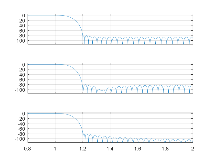
 clf; a=[.8 2 -115 5]; fc=1.1/pi; l="labelxy";
 for k=1:3; switch (k); case 1; w=kaiser(L=159, 7.91);
   case 2; w=ultrwin(L=165, 0, 2.73); case 3; w=ultrwin(L=153, .5, 2.6); end
   subplot(3, 1, 4-k); f=[1:(L-1)/2]*pi;f=sin(fc*f)./f; f=[fliplr(f) fc f]';
   [h,f]=freqz(w.*f,1,2^14); plot(f,20*log10(h)); grid; axis(a,l); l="labely";
 end
 %-----------------------------------------------------------
 % Figure shows example lowpass filter design (Fp=1, Fs=1.2
 % rad/s, att=80 dB) and comparison with other windows.  From
 % top to bottom: Ultraspherical, Dolph-Chebyshev, and Kaiser
 % windows, with lengths 153, 165, and 159 respectively.
Produces the following figure
| Figure 1 |
|---|
 |
Package: signal