- Function File: zplane
(z, p)¶ - Function File: zplane
(b, a)¶ Plot the poles and zeros on a complex plane. If the arguments are column vectors z and p, the complex zeros z and poles p are displayed. If the arguments are row vectors b and a, the zeros and poles of the transfer function represented by these filter coefficients are displayed.
If z and p are matrices, the columns are distinct sets of zeros and poles and are displayed together in distinct colors.
Note that due to the nature of the
rootsfunction, poles and zeros may be displayed as occurring around a circle rather than at a single point.The transfer function is
       B(z)   b0 + b1 z^(-1) + b2 z^(-2) + ... + bM z^(-M)
H(z) = ---- = --------------------------------------------
       A(z)   a0 + a1 z^(-1) + a2 z^(-2) + ... + aN z^(-N)

              b0          (z - z1) (z - z2) ... (z - zM)
            = -- z^(-M+N) ------------------------------
              a0          (z - p1) (z - p2) ... (z - pN)
If called with only one argument, the poles p defaults to an empty vector, and the denominator coefficient vector a defaults to 1.
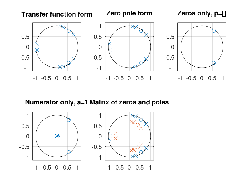
Demonstration 1
The following code
 ## construct target system:
 ##   symmetric zero-pole pairs at r*exp(iw),r*exp(-iw)
 ##   zero-pole singletons at s
 pw = [0.2, 0.4, 0.45, 0.95];   # pw = [0.4];
 pr = [0.98, 0.98, 0.98, 0.96]; # pr = [0.85];
 ps = [];
 zw = [0.3];  # zw=[];
 zr = [0.95]; # zr=[];
 zs = [];

 ## system function for target system
 p = [[pr, pr] .* exp(1i * pi * [pw, -pw]), ps]';
 z = [[zr, zr] .* exp(1i * pi * [zw, -zw]), zs]';
 M = length(z);
 N = length(p);
 sys_a = [zeros(1, M-N), real(poly(p))];
 sys_b = [zeros(1, N-M), real(poly(z))];

 disp ("The first two graphs should be identical, with poles at (r,w) =");
 disp (sprintf(" (%.2f,%.2f)", [pr; pw]));
 disp ("and zeros at (r,w) =");
 disp (sprintf(" (%.2f,%.2f)", [zr; zw]));
 disp ("with reflection across the horizontal axis");

 subplot (2, 3, 1);
 zplane (sys_b, sys_a);
 title ("Transfer function form");

 subplot (2, 3, 2);
 zplane (z, p);
 title ("Zero pole form");

 subplot (2, 3, 3);
 zplane (z);
 title ("Zeros only, p=[]");

 subplot (2, 3, 4);
 zplane (sys_b);
 title ("Numerator only, a=1");

 disp ("The matrix plot has 2 sets of points, one inside the other");
 subplot (2, 3, 5);
 zplane ([z, 0.7*z], [p, 0.7*p]);
 title ("Matrix of zeros and poles");
Produces the following output
The first two graphs should be identical, with poles at (r,w) =
 (0.98,0.20) (0.98,0.40) (0.98,0.45) (0.96,0.95)
and zeros at (r,w) =
 (0.95,0.30)
with reflection across the horizontal axis
The matrix plot has 2 sets of points, one inside the other
and the following figure
| Figure 1 |
|---|
 |
Package: signal