Function File: [yi p sigma2,unc_y] = csaps_sel(x, y, xi, w=[], crit=[]) ¶

Function File: [pp p sigma2,unc_y] = csaps_sel(x, y, [], w=[], crit=[]) ¶

Cubic spline approximation with smoothing parameter estimation
Approximately interpolates [x,y], weighted by w (inverse variance; if not given, equal weighting is assumed), at xi.

The chosen cubic spline with natural boundary conditions pp(x) minimizes p Sum_i w_i*(y_i - pp(x_i))^2 + (1-p) Int pp”(x) dx.

A selection criterion crit is used to find a suitable value for p (between 0 and 1); possible values for crit are ‘vm’ (Vapnik’s measure [Cherkassky and Mulier 2007] from statistical learning theory); ‘aicc’ (corrected Akaike information criterion, the default); ‘aic’ (original Akaike information criterion); ‘gcv’ (generalized cross validation).

If crit is a nonnegative scalar instead of a string, then p is chosen to so that the mean square scaled residual Mean_i (w_i*(y_i - pp(x_i))^2) is approximately equal to crit. If crit is a negative scalar, then p is chosen so that the effective number of degrees of freedom in the spline fit (which ranges from 2 when p = 0 to n when p = 1) is approximately equal to -crit.

x and w should be n by 1 in size; y should be n by m; xi should be k by 1; the values in x should be distinct and in ascending order; the values in w should be nonzero.

Returns the smoothing spline pp or its values yi at the desired xi; the selected p; the estimated data scatter (variance from the smooth trend) sigma2; the estimated uncertainty (SD) of the smoothing spline fit at each x value, unc_y; and the estimated number of degrees of freedom df (out of n) used in the fit.

For small n, the optimization uses singular value decomposition of an n by n matrix in order to quickly compute the residual size and model degrees of freedom for many p values for the optimization (Craven and Wahba 1979). For large n (currently >300), an asymptotically more computation and storage efficient method that takes advantage of the sparsity of the problem’s coefficient matrices is used (Hutchinson and de Hoog 1985).

References:

Vladimir Cherkassky and Filip Mulier (2007), Learning from Data: Concepts, Theory, and Methods. Wiley, Chapter 4

Carl de Boor (1978), A Practical Guide to Splines, Springer, Chapter XIV

Clifford M. Hurvich, Jeffrey S. Simonoff, Chih-Ling Tsai (1998), Smoothing parameter selection in nonparametric regression using an improved Akaike information criterion, J. Royal Statistical Society, 60B:271-293

M. F. Hutchinson and F. R. de Hoog (1985), Smoothing noisy data with spline functions, Numerische Mathematik, 47:99-106

M. F. Hutchinson (1986), Algorithm 642: A fast procedure for calculating minimum cross-validation cubic smoothing splines, ACM Transactions on Mathematical Software, 12:150-153

Grace Wahba (1983), Bayesian “confidence intervals” for the cross-validated smoothing spline, J Royal Statistical Society, 45B:133-150

Herman J. Woltring (1986), A Fortran package for generalized, cross-validatory spline smoothing and differentiation, Advances in Engineering Software, 8(2):104–113

See also: csaps, spline, csapi, ppval, dedup, bin_values, gcvspl.

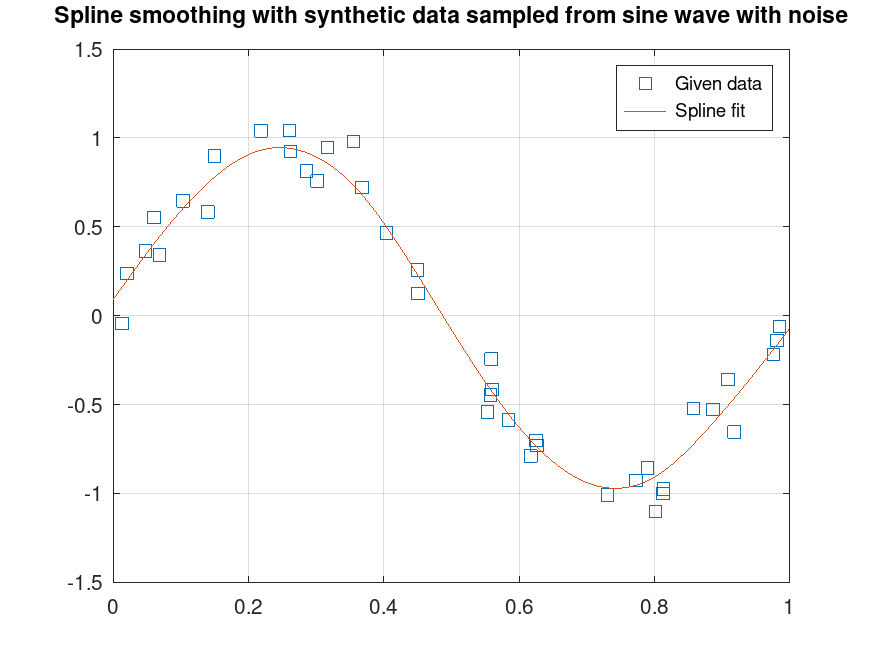
Demonstration 1

Package: splines