- Function File: [grid,u] = regularization (data, interval, N, F1) 
- Function File: [grid,u] = regularization (data, interval, N, F1, F2) 
-
Apply a Tikhonov regularization, the functional to be minimized is
F = FD + lambda1*F1 + lambda2*F2
= sum_(i=1)^M (y_i-u(x_i))^2 + lambda1*int_a^b (u’(x) - g1(x))^2 dx + lambda2*int_a^b (u”(x) - g2(x))^2 dxWith lambda1 = 0 and G2(x) = 0 this leads to a smoothing spline.
Parameters:
- data is a M*2 matrix with the x values in the first column and the y values in the second column.
- interval = [a,b] is the interval on which the regularization is applied.
- N is the number of subintervals of equal length. grid will consist of N+1 grid points.
- F1 is a structure containing the information on the first regularization term, integrating the square of the first derivative.
- F1.lambda is the value of the regularization parameter lambda1>=0.
- F1.g is the function handle for the function g1(x). If not provided G1=0 is used.
- F2 is a structure containing the information on the second regularization term, integrating the square of the second derivative. If F2 is not provided lambda2=0 is assumed.
- F2.lambda is the value of the regularization parameter lambda2>=0.
- F2.g is the function handle for the function g2(x). If not provided G2=0 is used.
Return values:
- grid is the grid on which u is evaluated. It consists of N+1 equidistant points on the interval.
- u are the values of the regularized approximation to the data evaluated at grid.
See also: csaps, regularization2D, demo regularization.
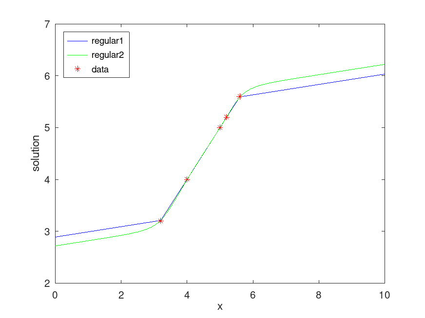
Demonstration 1
The following code
 N = 100;   interval = [0,10];
 x = [3.2,4,5,5.2,5.6]'; y = x;

 clear F1 F2
 %% regularize towards slope 0.1, no smoothing
 F1.lambda = 1e-2;   F1.g = @(x)0.1*ones(size(x));
 [grid,u1] = regularization([x,y],interval,N,F1);
 %% regularize towards slope 0.1, with some smoothing
 F2.lambda = 1*1e-3;
 [grid,u2] = regularization([x,y],interval,N,F1,F2);

 figure(1)
 plot(grid,u1,'b',grid,u2,'g',x,y,'*r')
 xlabel('x'); ylabel('solution');
 legend('regular1','regular2','data','location','northwest')
Produces the following figure
| Figure 1 |
|---|
 |
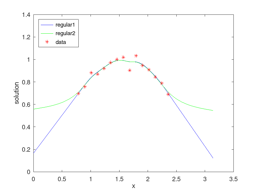
Demonstration 2
The following code
 N = 1000;   interval = [0,pi];
 x = linspace( pi/4,3*pi/4,15)';   y = sin(x)+ 0.03*randn(size(x));

 clear F1 F2
 %% regularize by smoothing only
 F1.lambda = 0;  F2.lambda = 1e-3;
 [grid,u1] = regularization([x,y],interval,N,F1,F2);
 %% regularize by smoothing and aim for slope 0
 F1.lambda = 1*1e-2;
 [grid,u2] = regularization([x,y],interval,N,F1,F2);

 figure(1)
 plot(grid,u1,'b',grid,u2,'g',x,y,'*r')
 xlabel('x'); ylabel('solution');
 legend('regular1','regular2','data','location','northwest')
Produces the following figure
| Figure 1 |
|---|
 |
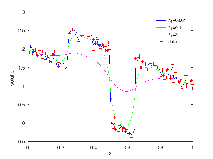
Demonstration 3
The following code
 interval = [0,1];
 N = 400;
 x = rand(200,1);
 %% generate the data on four line segments, add some noise
 y = 2 - 2*x + (x>0.25) - 2*(x>0.5).*(x<0.65)+ 0.1*randn(length(x),1);
 clear F1
 %% apply regularization with three different parameters
 F1.lambda = 1e-3; [grid,u1] = regularization([x,y],interval,N,F1);
 F1.lambda = 1e-1; [grid,u2] = regularization([x,y],interval,N,F1);
 F1.lambda = 3e+0; [grid,u3] = regularization([x,y],interval,N,F1);

 figure(1); plot(grid,u1,'b',grid,u2,'g',grid,u3,'m',x,y,'+r')
            xlabel('x'); ylabel('solution')
            legend('\lambda_1=0.001','\lambda_1=0.1','\lambda_1=3','data')
Produces the following figure
| Figure 1 |
|---|
 |
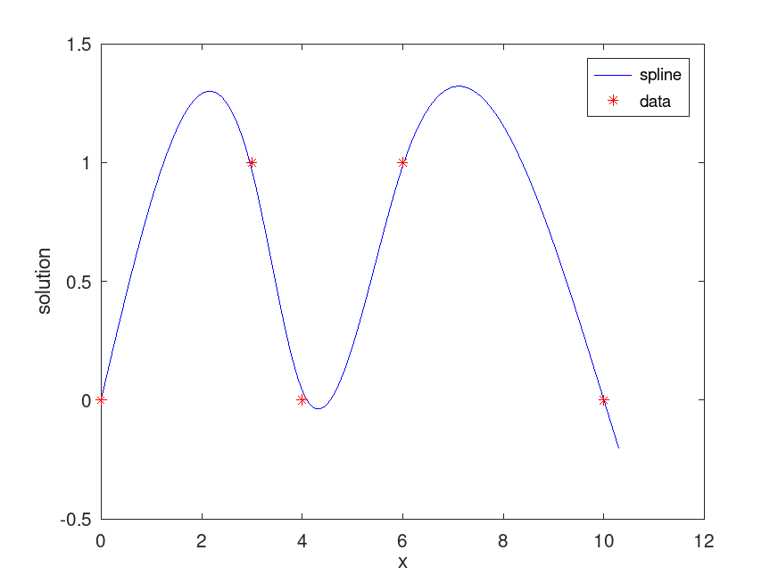
Demonstration 4
The following code
 %% generate a smoothing spline, see also csaps() in the package splines
 N = 1000;  interval = [0,10.3];
 x = [0 3 4 6 10]';  y = [0 1 0 1 0]';
 clear F2
 F2.lambda = 1e-2;
 %% apply regularization, the result is a smoothing spline
 [grid,u] = regularization([x,y],interval,N,0,F2);

 figure(1);
 plot(grid,u,'b',x,y,'*r')
 legend('spline','data')
 xlabel('x'); ylabel('solution')
Produces the following figure
| Figure 1 |
|---|
 |
Package: splines