- Function File: [grid,u,data_valid] = regularization2D (data, box, N, lambda1,lambda2) 
-
Apply a Tikhonov regularization, the functional to be minimized is
F = FD + lambda1 * F1 + lambda2 * F2
= sum_(i=1)^M (y_i-u(x_i))^2 +
+ lambda1 * dintegral (du/dx)^2+(du/dy)^2 dA +
+ lambda2 * dintegral (d^2u/dx^2)^2+(d^2u/dy^2)^2+2*(d^2u/dxdy) dAWith lambda1 = 0 and lambda2>0 this leads to a thin plate smoothing spline.
Parameters:
- data is a M*3 matrix with the (x,y) values in the first two columns and the y values in the third column.
Only data points strictly inside the box are used - box = [x0,x1;y0,y1] is the rectangle x0<x<x1 and y0<y<y1 on which the regularization is applied.
- N = [N1,N2] determines the number of subintervals of equal length. grid will consist of (N1+1)x(N2+1) grid points.
- lambda1 >= 0 is the value of the first regularization parameter
- lambda2 > 0 is the value of the secondregularization parameter
Return values:
- grid is the grid on which u is evaluated. It consists of (N1+1)x(N2+1) equidistant points on the the rectangle box.
- u are the values of the regularized approximation to the data evaluated on the grid.
- data_valid returns the values data points used and the values of the regularized function at these points
See also: tpaps, regularization, demo regularization2D.
- data is a M*3 matrix with the (x,y) values in the first two columns and the y values in the third column.
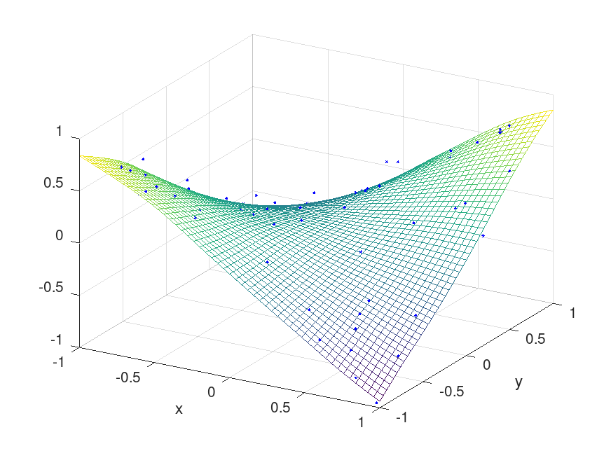
Demonstration 1
The following code
 M = 100;
 lambda1 = 0; lambda2 = 0.05;
 x = 2*rand(M,1)-1;     y = 2*rand(M,1)-1;
 z = x.*y + 0.1*randn(M,1);
 data = [x,y,z];
 [grid,u] = regularization2D(data,[-1 1;-1 1],[50 50],lambda1,lambda2);
 figure()
 mesh(grid.x, grid.y,u)
 xlabel('x'); ylabel('y');
 hold on
 plot3(data(:,1),data(:,2),data(:,3),'*b','Markersize',2)
 hold off
 view([30,30]);
Produces the following figure
| Figure 1 |
|---|
 |
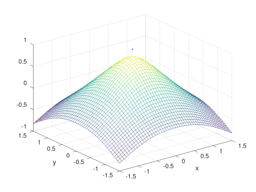
Demonstration 2
The following code
 lambda1 = 0; lambda2 = 0.01;
 M = 4;  angles = [1:M]/M*2*pi;
 data = zeros(M+1,3);  data(M+1,3) = 1;
 data(1:M,1) = cos(angles); data(1:M,2) = sin(angles);
 [grid,u] = regularization2D(data,[-1.5 1.5;-1.5 1.5],[50 50],lambda1,lambda2);
 figure()
 mesh(grid.x, grid.y,u)
 xlabel('x'); ylabel('y');
 hold on
 plot3(data(:,1),data(:,2),data(:,3),'*b','Markersize',2)
 hold off
Produces the following figure
| Figure 1 |
|---|
 |
Package: splines