- Function File: y = mvnpdf (x)
- Function File: y = mvnpdf (x, mu)
- Function File: y = mvnpdf (x, mu, sigma)
Compute multivariate normal pdf for x given mean mu and covariance matrix sigma. The dimension of x is d x p, mu is 1 x p and sigma is p x p. The normal pdf is defined as
1/y^2 = (2 pi)^p |Sigma|exp { (x-mu)' inv(Sigma) (x-mu) }References
NIST Engineering Statistics Handbook 6.5.4.2 http://www.itl.nist.gov/div898/handbook/pmc/section5/pmc542.htm
Algorithm
Using Cholesky factorization on the positive definite covariance matrix:
r = chol (sigma);
where r’*r = sigma. Being upper triangular, the determinant of r is trivially the product of the diagonal, and the determinant of sigma is the square of this:
det = prod (diag (r))^2;
The formula asks for the square root of the determinant, so no need to square it.
The exponential argument A = x’ * inv (sigma) * x
A = x' * inv (sigma) * x
  = x' * inv (r' * r) * x
  = x' * inv (r) * inv(r') * x
Given that inv (r’) == inv(r)’, at least in theory if not numerically,
A = (x' / r) * (x'/r)' = sumsq (x'/r)
The interface takes the parameters to the multivariate normal in columns rather than rows, so we are actually dealing with the transpose:
A = sumsq (x/r)
and the final result is:
r = chol (sigma)
y = (2*pi)^(-p/2) * exp (-sumsq ((x-mu)/r, 2)/2) / prod (diag (r))
See also: mvncdf, mvnrnd.
Demonstration 1
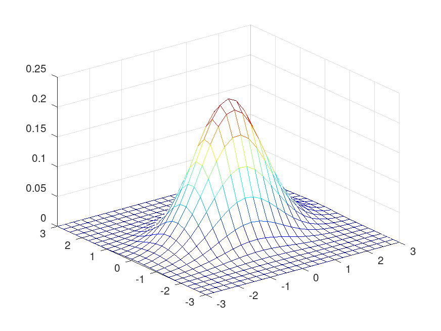
The following code
 mu = [0, 0];
 sigma = [1, 0.1; 0.1, 0.5];
 [X, Y] = meshgrid (linspace (-3, 3, 25));
 XY = [X(:), Y(:)];
 Z = mvnpdf (XY, mu, sigma);
 mesh (X, Y, reshape (Z, size (X)));
 colormap jet
Produces the following figure
| Figure 1 |
|---|
 |
Package: statistics