- Function File: [m, K] = regress_gp (x, y, Sp)
- Function File: [… yi dy] = regress_gp (…, xi)
Linear scalar regression using gaussian processes.
It estimates the model y = x’*m for x R^D and y in R. The information about errors of the predictions (interpolation/extrapolation) is given by the covarianve matrix K. If D==1 the inputs must be column vectors, if D>1 then x is n-by-D, with n the number of data points. Sp defines the prior covariance of m, it should be a (D+1)-by-(D+1) positive definite matrix, if it is empty, the default is
Sp = 100*eye(size(x,2)+1).If xi inputs are provided, the model is evaluated and returned in yi. The estimation of the variation of yi are given in dy.
Run
demo regress_gpto see an examples.The function is a direc implementation of the formulae in pages 11-12 of Gaussian Processes for Machine Learning. Carl Edward Rasmussen and Christopher K. I. Williams. The MIT Press, 2006. ISBN 0-262-18253-X. available online at http://gaussianprocess.org/gpml/.
See also: regress.
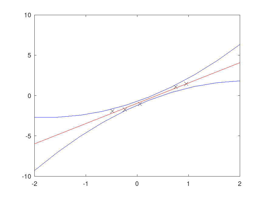
Demonstration 1
The following code
 % 1D Data
 x = 2*rand (5,1)-1;
 y = 2*x -1 + 0.3*randn (5,1);

 % Points for interpolation/extrapolation
 xi = linspace (-2,2,10)';

 [m K yi dy] = regress_gp (x,y,[],xi);

 plot (x,y,'xk',xi,yi,'r-',xi,bsxfun(@plus, yi, [-dy +dy]),'b-');
Produces the following figure
| Figure 1 |
|---|
 |
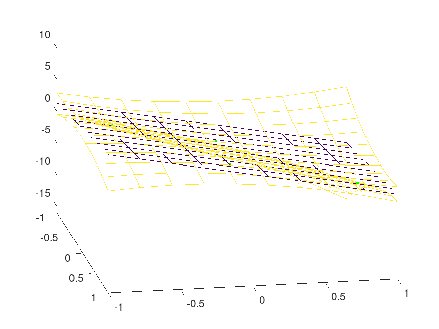
Demonstration 2
The following code
 % 2D Data
 x = 2*rand (4,2)-1;
 y = 2*x(:,1)-3*x(:,2) -1 + 1*randn (4,1);

 % Mesh for interpolation/extrapolation
 [xi yi] = meshgrid (linspace (-1,1,10));

 [m K zi dz] = regress_gp (x,y,[],[xi(:) yi(:)]);
 zi = reshape (zi, 10,10);
 dz = reshape (dz,10,10);

 plot3 (x(:,1),x(:,2),y,'.g','markersize',8);
 hold on;
 h = mesh (xi,yi,zi,zeros(10,10));
 set(h,'facecolor','none');
 h = mesh (xi,yi,zi+dz,ones(10,10));
 set(h,'facecolor','none');
 h = mesh (xi,yi,zi-dz,ones(10,10));
 set(h,'facecolor','none');
 hold off
 axis tight
 view(80,25)
Produces the following figure
| Figure 1 |
|---|
 |
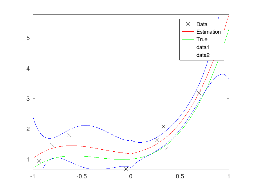
Demonstration 3
The following code
 % Projection over basis function
 pp = [2 2 0.3 1];
 n = 10;
 x = 2*rand (n,1)-1;
 y = polyval(pp,x) + 0.3*randn (n,1);

 % Powers
 px = [sqrt(abs(x)) x x.^2 x.^3];

 % Points for interpolation/extrapolation
 xi = linspace (-1,1,100)';
 pxi = [sqrt(abs(xi)) xi xi.^2 xi.^3];

 Sp      = 100*eye(size(px,2)+1);
 Sp(2,2) = 1; # We don't believe the sqrt is present
 [m K yi dy] = regress_gp (px,y,Sp,pxi);
 disp(m)

 plot (x,y,'xk;Data;',xi,yi,'r-;Estimation;',xi,polyval(pp,xi),'g-;True;');
 axis tight
 axis manual
 hold on
 plot (xi,bsxfun(@plus, yi, [-dy +dy]),'b-');
 hold off
Produces the following output
1.1572
   0.1989
   0.2314
   2.0433
   2.1448
and the following figure
| Figure 1 |
|---|
 |
Package: statistics