- : [smpl, neval] = slicesample (start, nsamples, property, value, …)
Draws nsamples samples from a target stationary distribution pdf using slice sampling of Radford M. Neal.
Input:
- start is a 1 by dim vector of the starting point of the Markov chain. Each column corresponds to a different dimension.
- nsamples is the number of samples, the length of the Markov chain.
Next, several property-value pairs can or must be specified, they are:
(Required properties) One of:
- "pdf": the value is a function handle of the target stationary
distribution to be sampled. The function should accept different locations
in each row and each column corresponds to a different dimension.
or
- logpdf: the value is a function handle of the log of the target stationary distribution to be sampled. The function should accept different locations in each row and each column corresponds to a different dimension.
The following input property/pair values may be needed depending on the desired outut:
- "burnin" burnin the number of points to discard at the beginning, the default is 0.
- "thin" thin omitts m-1 of every m points in the generated Markov chain. The default is 1.
- "width" width the maximum Manhattan distance between two samples. The default is 10.
Outputs:
- smpl is a nsamples by dim matrix of random values drawn from pdf where the rows are different random values, the columns correspond to the dimensions of pdf.
- neval is the number of function evaluations per sample.
Example : Sampling from a normal distribution
start = 1;
nsamples = 1e3;
pdf = @(x) exp (-.5 * x .^ 2) / (pi ^ .5 * 2 ^ .5);
[smpl, accept] = slicesample (start, nsamples, "pdf", pdf, "thin", 4);
histfit (smpl);
See also: rand, mhsample, randsample.
Demonstration 1
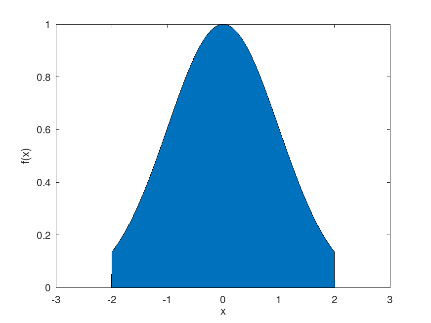
The following code
 ##Integrate truncated normal distribution to find normilization constant
 pdf = @(x) exp (-.5*x.^2)/(pi^.5*2^.5);
 nsamples = 1e3;
 [smpl,accept] = slicesample (1, nsamples, "pdf", pdf, "thin", 4);
 f = @(x) exp (-.5 * x .^ 2) .* (x >= -2 & x <= 2);
 x=linspace(-3,3,1000);
 area(x,f(x));
 xlabel ('x');
 ylabel ('f(x)');
 int = mean (f (smpl)./pdf(smpl));
 errest = std (f (smpl)./pdf(smpl))/nsamples^.5;
 trueerr = abs (erf (2^.5)*2^.5*pi^.5-int);
 fprintf("Monte Carlo integral estimate int f(x) dx = %f\n", int);
 fprintf("Monte Carlo integral error estimate %f\n", errest);
 fprintf("The actual error %f\n", trueerr);
Produces the following output
Monte Carlo integral estimate int f(x) dx = 2.366257
Monte Carlo integral error estimate 0.018234
The actual error 0.026319
and the following figure
| Figure 1 |
|---|
 |
Package: statistics