- wblplot.m: wblplot (data,...)
- wblplot.m: handle = wblplot (data,...)
- wblplot.m: [handle param] = wblplot (data)
- wblplot.m: [handle param] = wblplot (data , censor)
- wblplot.m: [handle param] = wblplot (data , censor, freq)
- wblplot.m: [handle param] = wblplot (data , censor, freq, confint)
- wblplot.m: [handle param] = wblplot (data , censor, freq, confint, fancygrid)
- wblplot.m: [handle param] = wblplot (data , censor, freq, confint, fancygrid, showlegend)
-
Plot a column vector data on a Weibull probability plot using rank regression.
censor: optional parameter is a column vector of same size as data with 1 for right censored data and 0 for exact observation. Pass [] when no censor data are available.
freq: optional vector same size as data with the number of occurences for corresponding data. Pass [] when no frequency data are available.
confint: optional confidence limits for ploting upper and lower confidence bands using beta binomial confidence bounds. If a single value is given this will be used such as LOW = a and HIGH = 1 - a. Pass [] if confidence bounds is not requested.
fancygrid: optional parameter which if set to anything but 1 will turn of the the fancy gridlines.
showlegend: optional parameter that when set to zero(0) turns off the legend.
If one output argument is given, a handle for the data marker and plotlines are returned which can be used for further modification of line and marker style.
If a second output argument is specified, a param vector with scale, shape and correlation factor is returned.
See also: normplot, wblpdf.
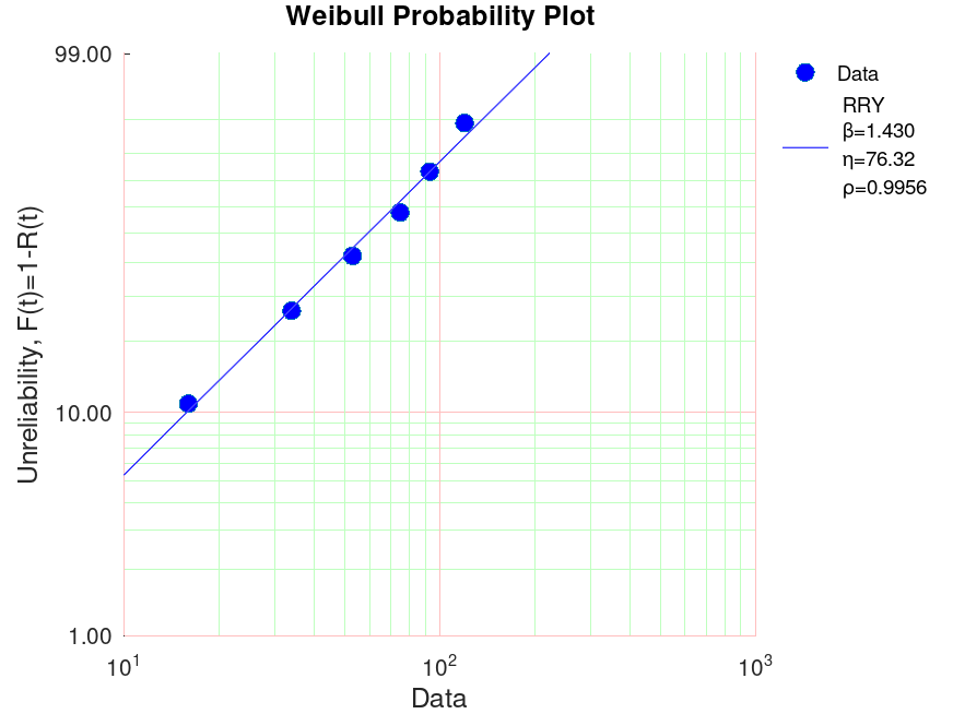
Demonstration 1
The following code
 x=[16 34 53 75 93 120];
 wblplot(x);
Produces the following figure
| Figure 1 |
|---|
 |
Demonstration 2
The following code
 x=[2 3 5 7 11 13 17 19 23 29 31 37 41 43 47 53 59 61 67]';
 c=[0 1 0 1 0 1 1 1 0 0 1 0 1 0 1 1 0 1 1]';
 [h p]=wblplot(x,c)
Produces the following output
h =

  -176.83
  -175.75

p =

   82.0192    0.8951    0.9896
and the following figure
| Figure 1 |
|---|
 |
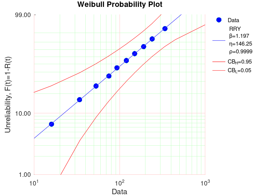
Demonstration 3
The following code
 x=[16, 34, 53, 75, 93, 120, 150, 191, 240 ,339];
 [h p]=wblplot(x,[],[],0.05)
 ## Benchmark Reliasoft eta = 146.2545 beta 1.1973 rho = 0.9999
Produces the following output
h =

  -176.30
  -175.19
  -174.49
  -173.65

p =

   146.2545     1.1973     0.9999
and the following figure
| Figure 1 |
|---|
 |
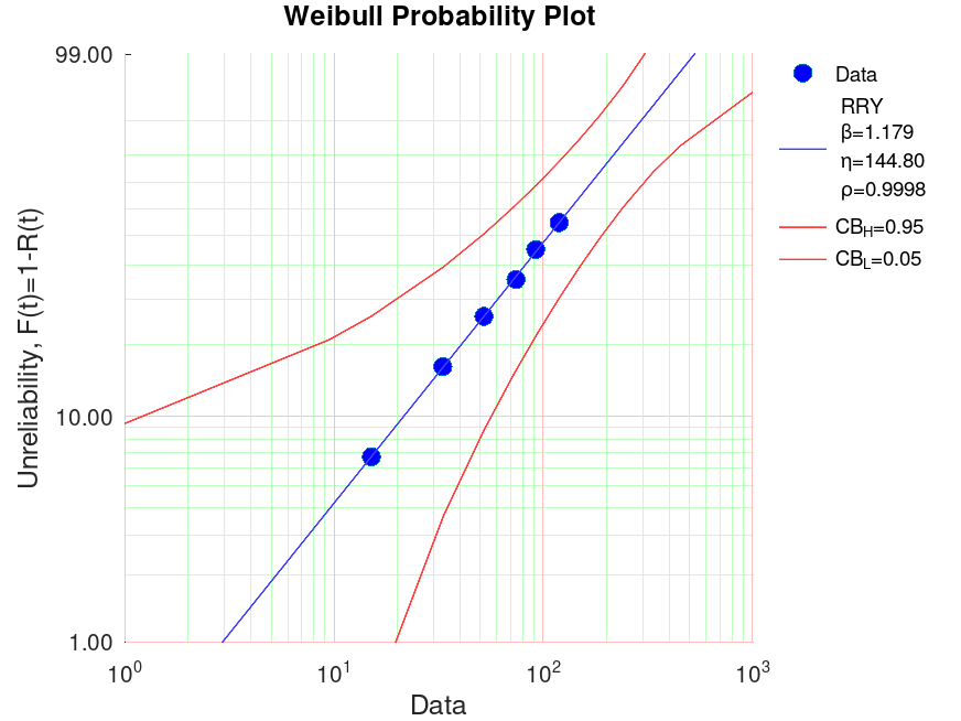
Demonstration 4
The following code
 x=[46 64 83 105 123 150 150];
 c=[0 0 0 0 0 0 1];
 f=[1 1 1 1 1 1 4];
 wblplot(x,c,f,0.05);
Produces the following figure
h =

  -176.30
  -175.19
  -174.49
  -173.65

p =

   146.2545     1.1973     0.9999
and the following figure
| Figure 1 |
|---|
 |
Demonstration 5
The following code
 x=[46 64 83 105 123 150 150];
 c=[0 0 0 0 0 0 1];
 f=[1 1 1 1 1 1 4];
 ## Subtract 30.92 from x to simulate a 3 parameter wbl with gamma = 30.92
 wblplot(x-30.92,c,f,0.05);
Produces the following figure
h =

  -176.30
  -175.19
  -174.49
  -173.65

p =

   146.2545     1.1973     0.9999
and the following figure
| Figure 1 |
|---|
 |
Package: statistics