3.4 Root Finding 
3.4.1 Interval Newton Method 
In numerical analysis, Newton’s method can find an approximation to a root of a function. Starting at a location x₀ the algorithms executes the following step to produce a better approximation:
x₁ = x₀ − f (x₀) / f’ (x₀)
The step can be interpreted geometrically as an intersection of the graph’s tangent with the x-axis. Eventually, this may converge to a single root. In interval analysis, we start with an interval x₀ and utilize the following interval Newton step:
x₁ = (mid (x₀) − f (mid (x₀)) / f’ (x₀)) ∩ x₀
Here we use the pivot element mid (x₀) and produce an enclosure of all possible tangents with the x-axis. In special cases the division with f' (x₀) yields two intervals and the algorithm bisects the search range. Eventually this algorithm produces enclosures for all possible roots of the function f in the interval x₀. The interval newton method is implemented by the function @infsup/fzero.
To produce the derivative of function f, the automatic differentiation from the symbolic package bears a helping hand. However, be careful since this may introduce numeric errors with coefficients.
f = @(x) sqrt (x) + (x + 1) .* cos (x);
pkg load symbolic
df = function_handle (diff (formula (f (sym ("x")))))
  ⇒ df =

   @(x) -(x + 1) .* sin (x) + cos (x) + 1 ./ (2 * sqrt (x))
fzero (f, infsup ("[0, 6]"), df)
  ⇒ ans ⊂ 2×1 interval vector

        [2.059, 2.0591]
       [4.3107, 4.3108]
We could find two roots in the interval [0, 6].
3.4.2 Bisection 
Consider the function f (x, y) = -(5*y - 20*y^3 + 16*y^5)^6 + (-(5*x - 20*x^3 + 16*x^5)^3 + 5*y - 20*y^3 + 16*y^5)^2, which has several roots in the area x, y ∈ [-1, 1].
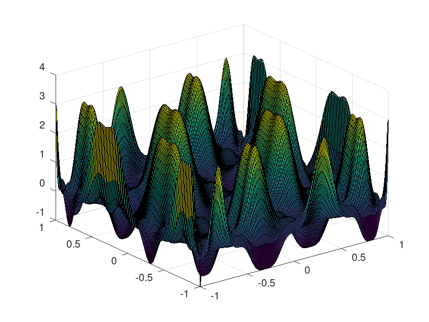 f (x, y) which shows a lot of roots for the function" />
The function is particular difficult to compute with intervals, because its variables appear several times in the expression, which benefits overestimation from the dependency problem. Computing root enclosures with the @infsup/fsolve function is unfeasible, because many bisections would be necessary until the algorithm terminates with a useful result. It is possible to reduce the overestimation with the @infsup/polyval function to some degree, but since this function is quite costly to compute, it does not speed up the bisecting algorithm.
f = @(x,y) ...
    -(5.*y - 20.*y.^3 + 16.*y.^5).^6 + ...
        (-(5.*x - 20.*x.^3 + 16.*x.^5).^3 + ...
           5.*y - 20.*y.^3 + 16.*y.^5).^2;
X = Y = infsup ("[-1, 1]");
has_roots = n = 1;
for iter = 1 : 10
    ## Bisect
    [i,j] = ind2sub ([n,n], has_roots);
    X = infsup ([X.inf,X.inf,X.mid,X.mid],[X.mid,X.mid,X.sup,X.sup]);
    Y = infsup ([Y.inf,Y.mid,Y.inf,Y.mid],[Y.mid,Y.sup,Y.mid,Y.sup]);
    ii = [2*(i-1)+1,2*(i-1)+2,2*(i-1)+1,2*(i-1)+2] ;
    jj = [2*(j-1)+1,2*(j-1)+1,2*(j-1)+2,2*(j-1)+2] ;
    has_roots = sub2ind ([2*n,2*n], ii, jj);
    n *= 2;

    ## Check if function value covers zero
    fval = f (X, Y);
    zero_contained = find (ismember (0, fval));

    ## Discard values without roots
    has_roots = has_roots(zero_contained);
    X = X(zero_contained);
    Y = Y(zero_contained);
endfor
colormap gray
B = false (n);
B(has_roots) = true;
imagesc (B)
axis equal
axis off
 f (x, y)" />
Now we use the same algorithm with the same number of iterations, but also utilize the mean value theorem to produce better enclosures of the function value with first order approximation of the function. The function is evaluated at the interval’s midpoint and a range evaluation of the derivative can be used to produce an enclosure of possible function values.
f_dx = @(x,y) ...
       -6.*(5 - 60.*x.^2 + 80.*x.^4) .* ...
           (5.*x - 20.*x.^3 + 16.*x.^5).^2 .* ...
           (-(5.*x - 20.*x.^3 + 16.*x.^5).^3 + ...
                5.*y - 20.*y.^3 + 16.*y.^5);
f_dy = @(x,y) ...
       -6.*(5 - 60.*y.^2 + 80.*y.^4) .* ...
           (5.*y - 20.*y.^3 + 16.*y.^5).^5 + ...
       2.*(5 - 60.*y.^2 + 80.*y.^4) .* ...
          (-(5.*x - 20.*x.^3 + 16.*x.^5).^3 + ...
                5.*y - 20.*y.^3 + 16.*y.^5);
for iter = 1 : 10
    ...
    ## Check if function value covers zero
    fval1 = f (X, Y);
    fval2 = f (mid (X), mid (Y)) + ...
            (X - mid (X)) .* f_dx (X, Y) + ...
            (Y - mid (Y)) .* f_dy (X, Y);
    fval = intersect (fval1, fval2);
    ...
endfor
By using the derivative, it is possible to reduce overestimation errors and achieve a much better convergence behavior.
 f (x, y)" />