3.5 Parameter Estimation 
3.5.1 Small Search Space 
Consider the model y (t) = p1 * exp (p2 * t). The parameters p1 and p2 are unknown, but it is known that the model fulfills the following constraints, which have been obtained using measurements with known error bounds.
p1, p2  ∈   [-3, 3]
y (0.2) ∈  [1.5, 2]
y (1)   ∈  [0.7, 0.8]
y (2)   ∈  [0.1, 0.3]
y (4)   ∈ [-0.1, 0.03]
A better enclosure of the parameters p1 and p2 can be estimated with the @infsup/fsolve function.
## Model
y = @(p1, p2, t) p1 .* exp (p2 .* t);
## Observations / Constraints
t = [0.2; 1; 2; 4];
y_t = infsup ("[1.5, 2]; [0.7, 0.8]; [0.1, 0.3]; [-0.1, 0.03]");
## Estimate parameters
f = @(p1, p2) y (p1, p2, t);
p = fsolve (f, infsup ("[-3, 3]; [-3, 3]"), y_t)
  ⇒ p ⊂ 2×1 interval vector

         [1.9863, 2.6075]
       [-1.3243, -1.0429]
The resulting p guarantees to contain all parameters [p1; p2] which satisfy all constraints on y. It is no surprise that f (p) intersects the constraints for y.
f (p(1), p(2))
  ⇒ ans ⊂ 4×1 interval vector

            [1.5241, 2.1166]
          [0.52838, 0.91888]
          [0.14055, 0.32382]
       [0.0099459, 0.040216]
3.5.2 Larger Search Space 
Consider the function f (x) = p1 ^ x * (p2 + p3 * x + p4 * x^2). Let’s say we have some known function values (measurements) and want to find matching parameters p1 through p4. The data sets (x, y) can be simulated. The parameters shall be reconstructed from the observed values on the search range p.
Using plain @infsup/fsolve would take considerably longer, because the search range has 4 dimensions. Bisecting intervals requires an exponential number of steps and can easily become inefficient. Thus we use a contractor for function f, which in addition to the function value can produce a refinement for its parameter constraints. Contractors can easily be build using interval reverse operations like @infsup/mulrev, @infsup/sqrrev, @infsup/powrev1, etc.
## Simulate some data sets and add uncertainty
x = -6 : 3 : 18;
f = @(p1, p2, p3, p4) ...
    p1 .^ x .* (p2 + p3 .* x + p4 .* x .^ 2);
y = f (1.5, 1, -3, 0.5) .* infsup ("[0.999, 1.001]");
function [fval, p1, p2, p3, p4] = ...
    contractor (y, p1, p2, p3, p4)
    x = -6 : 3 : 18;
    ## Forward evaluation
    a = p1 .^ x;
    b = p3 .* x;
    c = p2 + b;
    d = p4 .* x .^ 2;
    e = c + d;
    fval = a .* e;
    ## Reverse evaluation and
    ## undo broadcasting of x
    y = intersect (y, fval);
    a = mulrev (e, y, a);
    e = mulrev (a, y, e);
    p1 = powrev1 (x, a, p1);
    p1 = intersect (p1, [], 2);
    c = intersect (c, e - d);
    d = intersect (d, e - c);
    p2 = intersect (p2, c - b);
    p2 = intersect (p2, [], 2);
    b = intersect (b, c - p2);
    p3 = mulrev (x, b, p3);
    p3 = intersect (p3, [], 2);
    p4 = mulrev (x .^ 2, d, p4);
    p4 = intersect (p4, [], 2);
endfunction
Now, search for solutions in the range of p and try to restore the function parameters.
p = infsup ("[1.1, 2] [1, 5] [-5, -1] [0.1, 5]");
p = fsolve (@contractor, ...
            p, y, ...
            struct ("Contract", true))'
  ⇒ p ⊂ 4×1 interval vector

         [1.4991, 1.5009]
              [1, 1.0011]
       [-3.0117, -2.9915]
       [0.49772, 0.50578]
The function parameters 1.5, 1, −3, and 0.5 from above could be restored. The contractor function could significantly improve the convergence speed of the algorithm.
3.5.3 Combination of Functions 
Sometimes it is hard to express the search range in terms of a single function and its constraints, when the preimage of the function consists of a union or intersection of different parts. Several contractor functions can be combined using ctc_union or ctc_intersect to make a contractor function for more complicated sets. The combined contractor function allows one to solve for more complicated sets in a single step.
## General ring contractor
function [fval, cx1, cx2] = ctc_ring (y, c1, c2, x1, x2)
    ## Forward evaluation
    x1_c1 = x1 - c1;
    x2_c2 = x2 - c2;
    sqr_x1_c1 = x1_c1 .^ 2;
    sqr_x2_c2 = x2_c2 .^ 2;
    fval = hypot (x1_c1, x2_c2);
    ## Reverse evaluation
    y = intersect (y, fval);
    sqr_y = y .^ 2;
    sqr_x1_c1 = intersect (sqr_x1_c1, sqr_y - sqr_x2_c2);
    sqr_x2_c2 = intersect (sqr_x2_c2, sqr_y - sqr_x1_c1);
    x1_c1 = sqrrev (sqr_x1_c1, x1_c1);
    x2_c2 = sqrrev (sqr_x2_c2, x2_c2);
    cx1 = intersect (x1, x1_c1 + c1);
    cx2 = intersect (x2, x2_c2 + c2);
endfunction
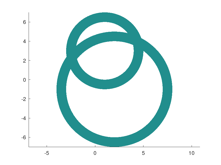
## Ring 1 with center at (1, 3)
## Ring 2 with center at (2, -1)
ctc_ring1 = @(y, x1, x2) ctc_ring (y, 1, 3, x1, x2);
ctc_ring2 = @(y, x1, x2) ctc_ring (y, 2, -1, x1, x2);
## Unite ring 1 with radius 3..4 and ring 2 with radius 5..6
ctc_union_of_rings = ctc_union (ctc_ring1, "[3, 4]", ...
                                ctc_ring2, "[5, 6]");
## Compute a paving to approximate the union of rings
## in the area x, y = -10..10
[~, paving] = fsolve (ctc_union_of_rings, ...
                      infsup ("[-10, 10] [-10, 10]"), ...
                      struct ("Contract", true));
plot (paving(1, :), paving(2, :))
axis equal

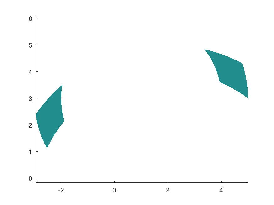
Intersections of contractor functions are especially useful to apply several constraints at once. For example, when it is known that a particular location has a distance of a ∈ [3, 4] from object A, located at coordinates (1, 3), and a distance of b ∈ [5, 6] from object B, located at coordinates (2, -1), the intersection of both rings yields all possible locations in the search range. The combined contractor function enables fast convergence of the search algorithm.
## Intersect ring 1 with radius 3..4 and ring 2 with radius 5..6
ctc_intersection_of_rings = ctc_intersect (ctc_ring1, "[3, 4]", ...
                                           ctc_ring2, "[5, 6]");
## Compute a paving to approximate the intersection of rings
## in the area x, y = -10..10
[~, paving] = fsolve (ctc_intersection_of_rings, ...
                      infsup ("[-10, 10] [-10, 10]"), ...
                      struct ("Contract", true));
plot (paving(1, :), paving(2, :))
axis equal
