
|
Octave-Forge - Extra packages for GNU Octave |
| Home · Packages · Developers · Documentation · FAQ · Bugs · Mailing Lists · Links · Code |
|
|
Octave-Forge - Extra packages for GNU Octave |
| Home · Packages · Developers · Documentation · FAQ · Bugs · Mailing Lists · Links · Code |
Solve the Eikonal equation using the Fast-Marching Method. In particular, the equation
|grad u |= f
is solved on a multi-dimensional domain. u0 and f must be multi-dimensional arrays of the same dimension and size, and the returned solution u will be also of this size. f should be positive, and we assume the grid spacing is unity (or, equivalently, has been absorbed into f already).
u0 defines the initial setting and the domain. It should contain the
initial distances for points that are used as initially alive points,
be Inf for points not part of the domain, and NA at all
other points. The latter are considered as far-away at the beginning
and their distances will be calculated. f is ignored at all but
the far-away points.
If g0 is also given, it should contain function values on initially alive points that will be extended onto the domain along the “normal directions”. This means that
grad g * grad u = 0
will be fulfilled for the solution u of the Eikonal equation.
g will be NA at points not in the domain or not reached by the
fast marching.
At return, u will contain the calculated distances.
Inf values will be retained, and it may still contain NA
at points to which no suitable path can be found.
See also: ls_signed_distance, ls_solve_stationary.
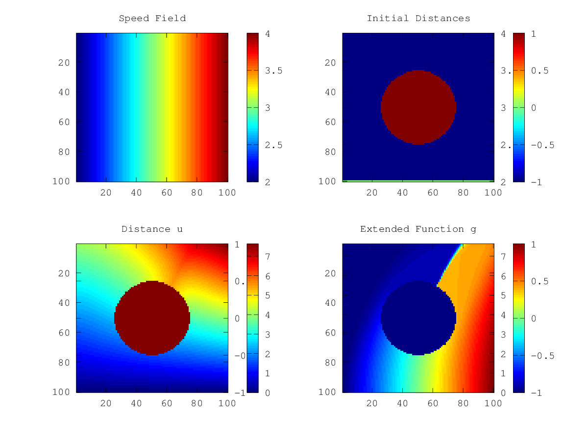
The following code
  n = 100;
  x = linspace (-1, 1, n);
  h = x(2) - x(1);
  [XX, YY] = meshgrid (x, x);

  u0 = NA (size (XX));
  u0(sqrt (XX.^2 + YY.^2) < 0.5) = Inf;
  u0(end, :) = 0;
  f = 3 + XX;
  g0 = NA (size (XX));
  g0(end, :) = x;

  [u, g] = fastmarching (u0, g0, h * f);

  figure ();
  subplot (2, 2, 1);
  imagesc (f);
  colorbar ();
  title ("Speed Field");
  subplot (2, 2, 2);
  imagesc (u0);
  colorbar ();
  title ("Initial Distances");
  subplot (2, 2, 3);
  imagesc (u);
  colorbar ();
  title ("Distance u");
  subplot (2, 2, 4);
  imagesc (g);
  colorbar ();
  title ("Extended Function g");
Produces the following figure
| Figure 1 |
|---|
 |
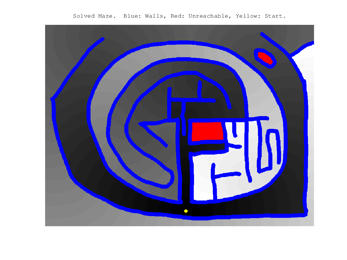
The following code
  pkgs = pkg ("list");
  file = false;
  for i = 1 : length (pkgs)
    if (strcmp (pkgs{i}.name, "level-set"))
      file = fullfile (pkgs{i}.dir, "maze.png");
    endif
  endfor
  if (!file)
    error ("could not locate example image file");
  endif
  img = double (imread (file)) / 255;

  % Red is the start area, white (not black) the accessible domain.
  start = (img(:, :, 1) > img(:, :, 2) + img(:, :, 3));
  domain = (img(:, :, 2) + img(:, :, 3) > 1.0) | start;

  u0 = NA (size (domain));
  u0(start) = 0;
  u0(~domain) = Inf;
  f = ones (size (u0));

  u = fastmarching (u0, f);
  u = u / max (u(isfinite (u)));

  % Format result as image.
  walls = isinf (u);
  notReached = isna (u);
  ur = u;
  ug = u;
  ub = u;
  ur(notReached) = 1;
  ug(notReached) = 0;
  ub(notReached) = 0;
  ur(walls) = 0;
  ug(walls) = 0;
  ub(walls) = 1;
  ur(start) = 1;
  ug(start) = 1;
  ub(start) = 0;
  u = NA (size (u, 1), size (u, 2), 3);
  u(:, :, 1) = ur;
  u(:, :, 2) = ug;
  u(:, :, 3) = ub;
  figure ();
  imshow (u);
  title ("Solved Maze.  Blue: Walls, Red: Unreachable, Yellow: Start.");
Produces the following figure
| Figure 1 |
|---|
 |
Package: level-set