
|
Octave-Forge - Extra packages for GNU Octave |
| Home · Packages · Developers · Documentation · FAQ · Bugs · Mailing Lists · Links · Code |
|
|
Octave-Forge - Extra packages for GNU Octave |
| Home · Packages · Developers · Documentation · FAQ · Bugs · Mailing Lists · Links · Code |
Solve a generalised Eikonal equation with speeds of arbitrary signs. The equation solved is
f |grad d |= 1
with d = 0 on the boundary. The domain is described by the level-set
function phi on a rectangular grid. f should contain the values
of the speed field on the grid points. h can be given as the
grid spacing. In the second form, where the optional nb is given,
it is used to initialise the narrow band with a manual calculation.
By default, the result of ls_init_narrowband is used. Values which
are not fixed by the narrow band should be set to NA.
Note that in comparison to fastmarching, the speed need not be
positive. It is the reciprocal of f in fastmarching.
This is a preparation step, and afterwards, the evolved geometry according to the level-set equation
d/dt phi + f |grad phi |= 0
can be extracted from d at arbitrary positive times using
the supplemental function ls_extract_solution.
At points where f is exactly zero, the output will be set
to NA. This case is handled separately in ls_extract_solution.
In the narrow band, the returned distances may actually be negative
even for positive f and vice-versa. This helps to avoid
unnecessary errors introduced into the level-set function due to
a finite grid-size when the time step is chosen small.
See also: ls_extract_solution, ls_signed_distance, ls_nb_from_geom.
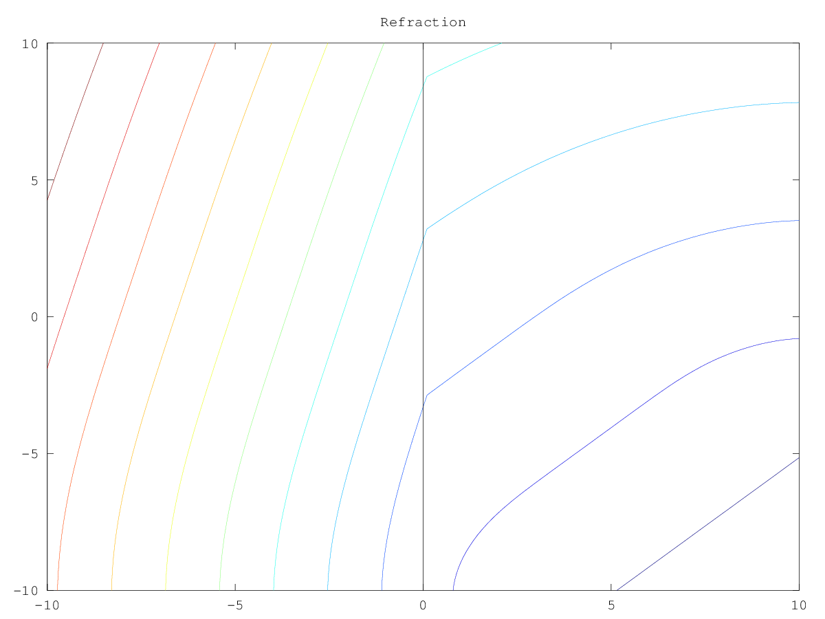
The following code
  n = 100;
  x = linspace (-10, 10, n);
  h = x(2) - x(1);
  [XX, YY] = meshgrid (x, x);

  phi0 = YY - XX + 15;
  f = sign (XX) + 2;

  d = ls_solve_stationary (phi0, f, h);
  figure ();
  contour (XX, YY, d);
  line ([0, 0], [-10, 10]);
  title ("Refraction");
Produces the following figure
| Figure 1 |
|---|
 |
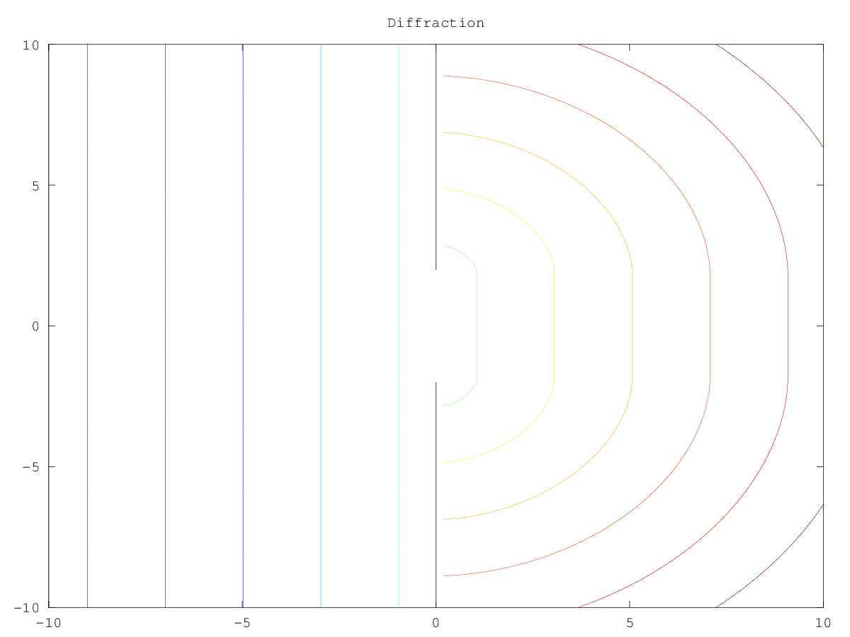
The following code
  n = 101;
  x = linspace (-10, 10, n);
  h = x(2) - x(1);
  [XX, YY] = meshgrid (x, x);

  phi0 = XX + 9;
  f = ones (size (phi0));
  f(XX == 0 & abs (YY) > 2) = 0;

  d = ls_solve_stationary (phi0, f, h);
  figure ();
  contour (XX, YY, d);
  line ([0, 0], [-10, -2]);
  line ([0, 0], [2, 10]);
  title ("Diffraction");
Produces the following figure
| Figure 1 |
|---|
 |
Package: level-set