
|
Octave-Forge - Extra packages for GNU Octave |
| Home · Packages · Developers · Documentation · FAQ · Bugs · Mailing Lists · Links · Code |
|
|
Octave-Forge - Extra packages for GNU Octave |
| Home · Packages · Developers · Documentation · FAQ · Bugs · Mailing Lists · Links · Code |
Run a descent method for shape optimisation. This routine is quite
general, since the actual “descent direction” used must be computed
by a callback (see below). It is thus not just for steepest descent.
At each step, a line search according to so_step_armijo is employed.
nSteps defines the maximal number of descent steps to take. After this number, the method returns no matter whether or not the stopping criterion is fulfilled. phi0 is the initial geometry to use. Returned are the final state and the descent log structs (see below).
data contains all the information about the actual problem. This includes various parameters that influence the behaviour of this and other routines. Furthermore, also some callback functions must be defined to evaluate the cost functional and to determine the next descent direction. This struct is also updated with the current state at each optimisation step and passed to the callback functions.
Most content of data is read-only, with data.s and
data.log being the only exceptions. They are updated
accordingly from the results of the callback functions and the
optimisation descent. These two structs will be created and filled in
by so_run_descent. data.log is preserved if it is
already present. data.s will always be overwritten
with the initial result of the update_state callback.
The struct data.p contains parameters. They can contain
problem-dependent parameters that are handled by the callback routines
as well as parameters for the line search with so_step_armijo.
This routine is influenced by the following parameters directly:
verboseWhether or not log chatter should be printed.
descent.initialStepInitial trial step length for the line search in the first iteration.
descent.projectSpeedIf set, project the speed field (in L2, discontinuously) to enforce geometric constraints (see below). If not set or missing, the geometry is projected instead.
The routine so_init_params can be used to initialise the parameter
structure with some defaults.
Information about the used grid and grid-dependent data should be in
data.g. Generally defined are the following fields:
hThe grid spacing.
constraintsOptional, can be used to specify the hold-all domain and contained
regions as shape constraints. If specified, the shape or the speed
field will be “projected” (depending on
data.p.descent.projectSpeed) to satisfy the constraints.
The callback computing the descent direction is also a good place
to take the constraints into account in a problem-specific way.
The following fields (as logical arrays with the grid size) can be used to specify the constraints:
holdallThe hold-all domain. The current shape must always be part of it. By excluding interior parts of the grid, forbidden regions can be defined.
containedA part of the hold-all domain that should always be part of the shape.
The specific problem is handled by callback routines to compute
the cost and find descent directions. They must be set in
data.cb, with these interfaces:
s = update_state (phi, data)Compute the state (see below) for the geometry described by phi.
The main work done by this callback is evaluating the cost functional.
It does not need to update s.phi to phi, this will
be done automatically after the call.
[f, dJ] = get_direction (data)Compute the speed field f and its associated directional
shape derivative dJ to be used as the next descent direction.
The current cost and geometry can be extracted from data.s.
exit = check_stop (data)Determine whether or not to stop the iteration. Should return
true if the state in data satisfies the problem-specific
stopping criterion. If not present, no stopping criterion
is used and the iteration done for precisely nSteps iterations.
d = solve_stationary (f, data)Solve the stationary Eikonal equation for the speed field.
If not present, ls_solve_stationary is used. It can be
set explicitly to give a more appropriate routine. For instance,
ls_nb_from_geom could be used if geometry information is computed.
Additional callback functions can be defined optionally
in data.handler. They can keep problem-specific
logs of the descent, plot figures, print output or something else.
They should always return a (possibly) updated log struct, which
will be updated in data.log after the call.
This struct can also be used to persist information between
calls to the handlers. These handlers can be defined:
log = initialised (data)Called before the iteration is started. data.s
contains the initial geometry and computed state data for it.
log = before_step (k, data)Called when starting a new step, before any action for the
step is taken. k is the number of the iteration and
data.s contains the current state.
log = direction (k, f, dJ, data)Called when the descent direction has been determined.
f and dJ are the results of data.cb.get_direction.
log = after_step (k, t, s, data)Called after a step has been found. t is the step length
found by the line search. s is the state struct after the step
has been taken. The previous state can still be found in
data.s.
log = finished (data)Called after the descent run. data.log is already filled
in with the standard data (number of steps and costs at each step).
Note that information about the speed field f is only
passed to the direction handler and not again
to after_step. If it is required by the latter,
it should be saved somehow in the log struct. This way, the handlers
really only receive new information and no redundant arguments.
Finally, we come to the state struct data.s. It must
contain at least the fields below, but can also contain problem-specific
information that is, for instance, computed in the update_state
handler and reused for computing the descent direction.
phiThe level-set function of the current geometry. This is automatically
updated after the update_state handler has been called.
costValue of the cost functional for the geometry in data.s.phi.
The log struct can contain mostly user-defined data, but
so_run_descent will also fill in some data by itself:
s0The state struct corresponding to the initial geometry defined by phi0.
stepsTotal number of steps done. This is useful if the stopping criterion was satisfied before nSteps iterations.
costsCost values for all steps. This will be a vector of length
data.log.steps + 1, since it contains both the initial
and the final cost value in addition to all intermediate ones.
See also: so_init_params, so_save_descent, so_replay_descent, so_explore_descent, so_step_armijo.
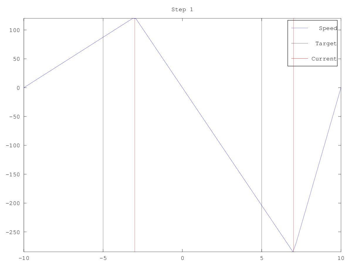
The following code
data = struct ();
data.p = so_init_params (true);
data.p.vol = 10;
data.p.weight = 50;
n = 100;
x = linspace (-10, 10, n);
h = x(2) - x(1);
data.g = struct ("x", x, "h", h);
% Look at so_example_problem to see how the callbacks
% and the plotting handler is defined.
data = so_example_problem (data);
phi0 = ls_genbasic (data.g.x, "box", -3, 7);
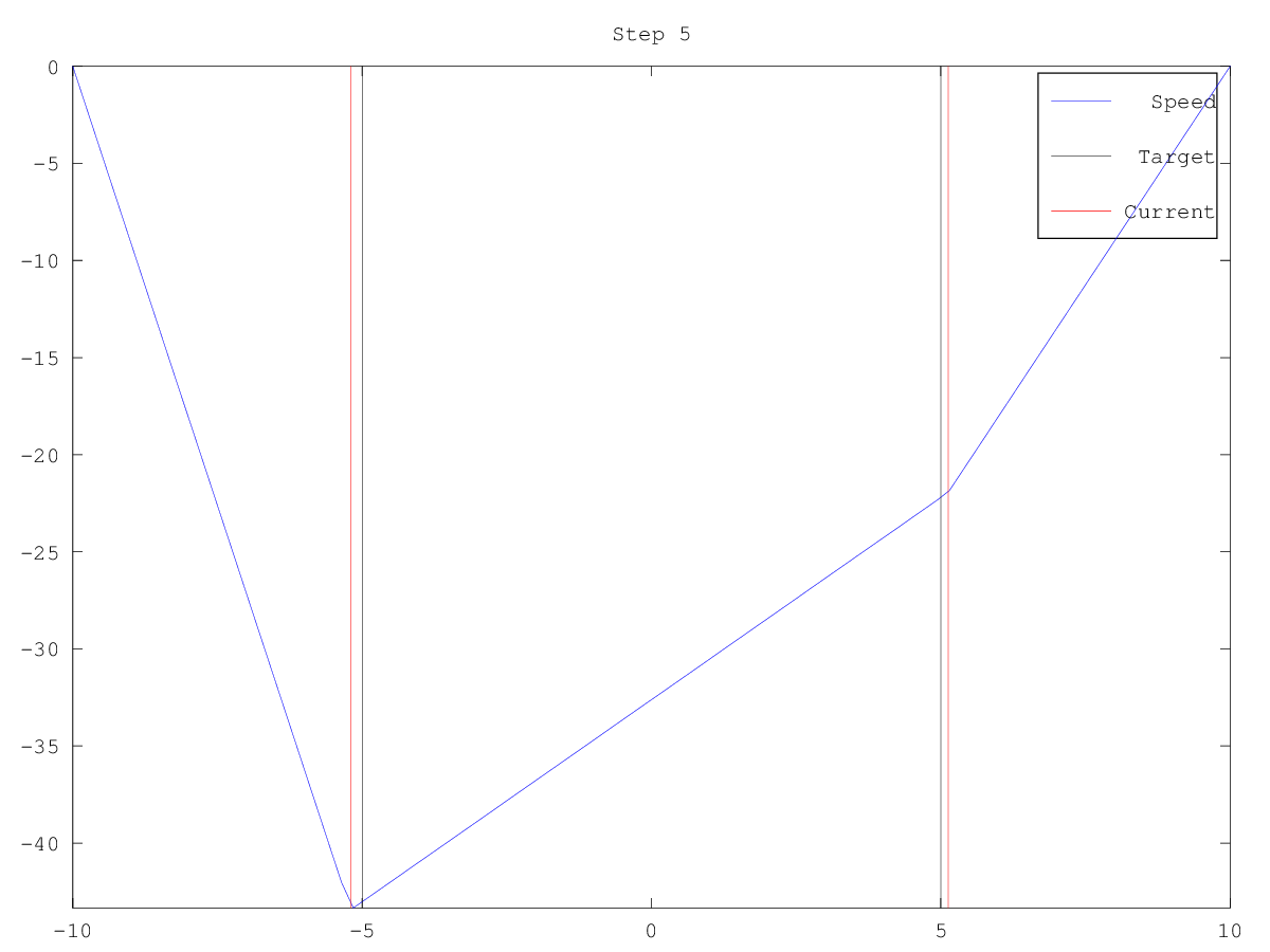
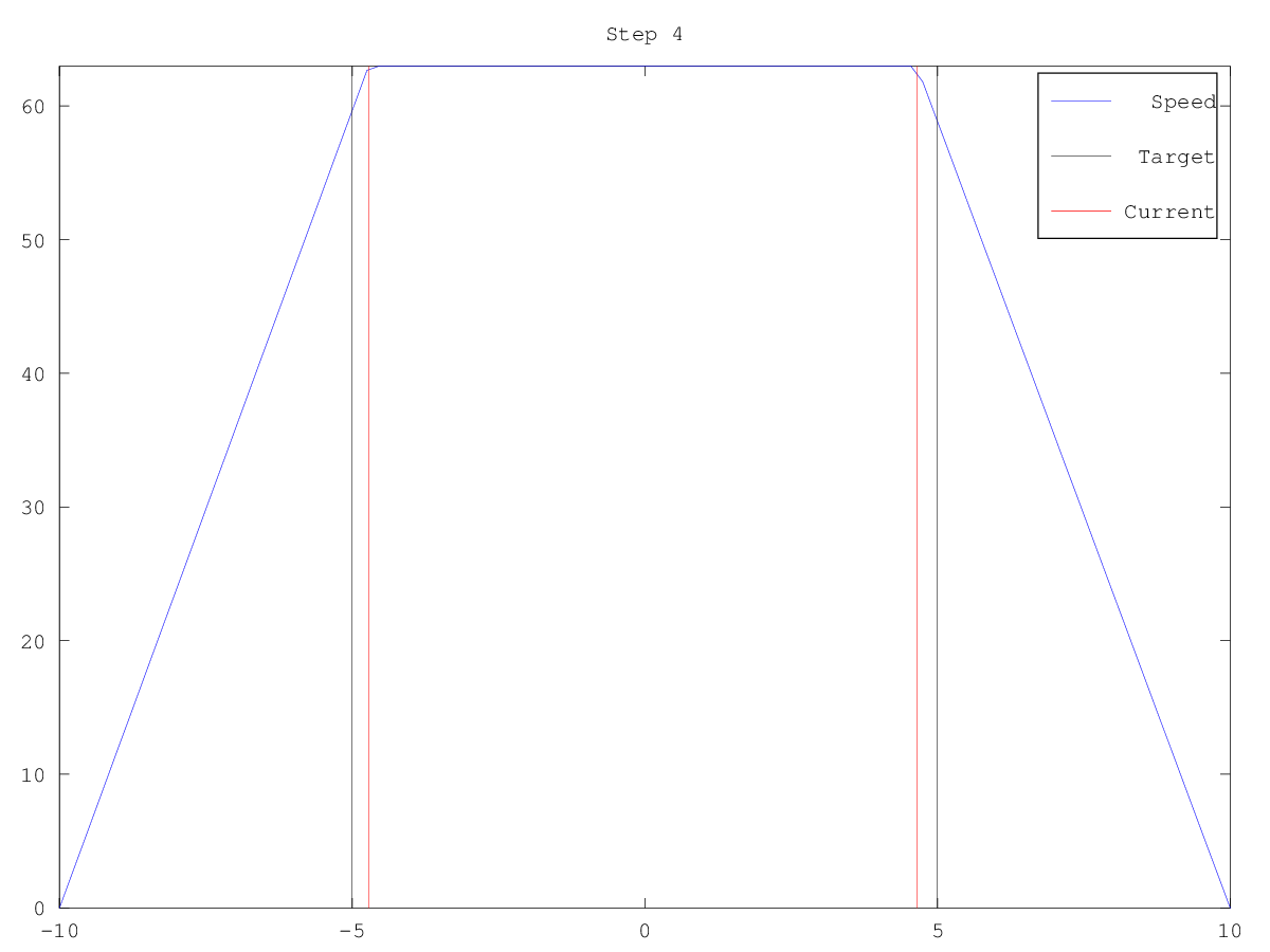
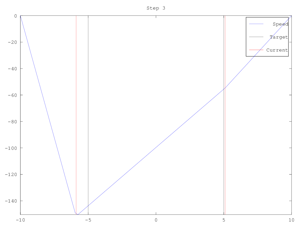
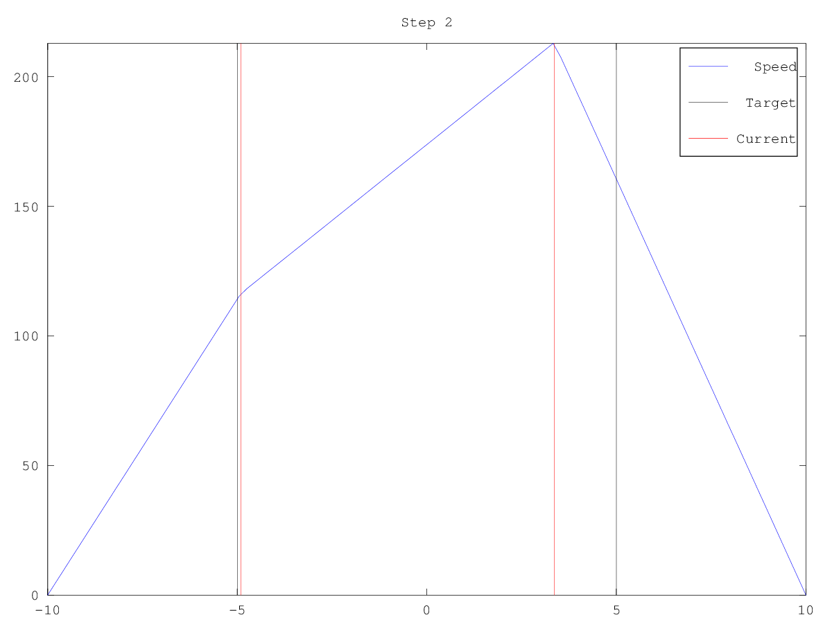
[s, descentLog] = so_run_descent (5, phi0, data);
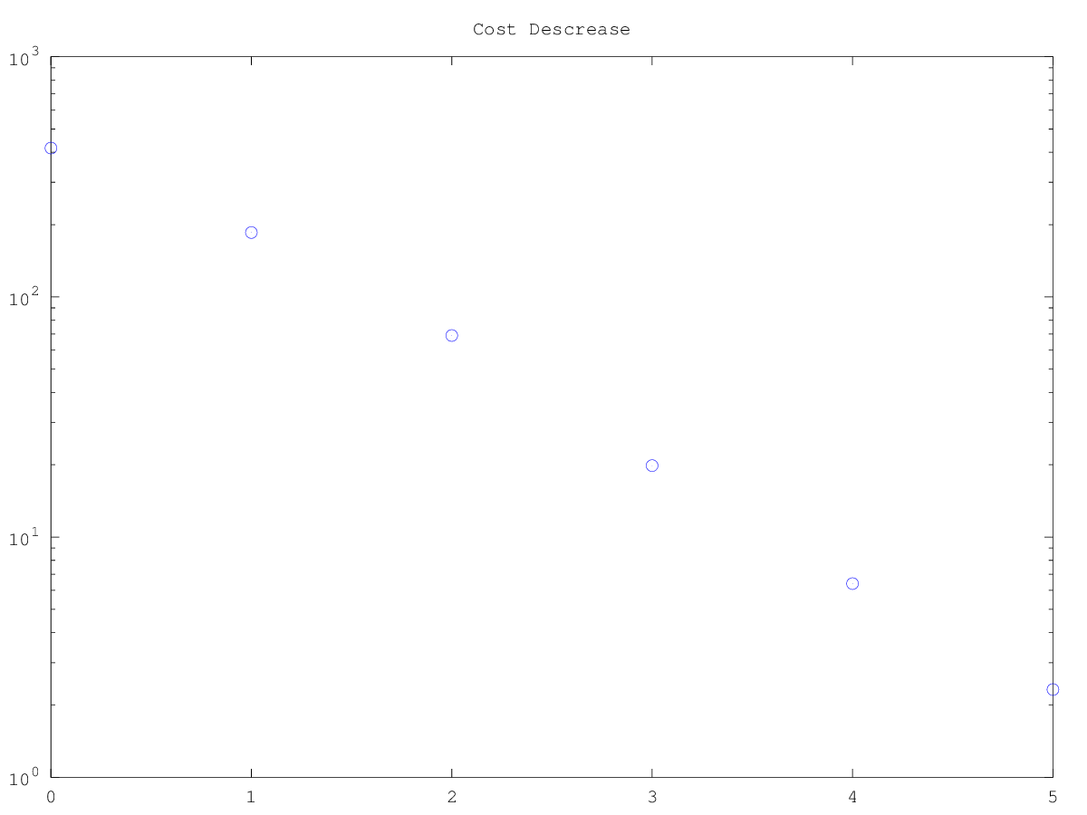
figure ();
semilogy (0 : descentLog.steps, descentLog.costs, "o");
title ("Cost Descrease");
printf ("\nFinal interval: [%.6d, %.6d]\n", s.a, s.b);
printf ("Final cost: %.6d\n", s.cost);
Produces the following output
Descent iteration 1...
Starting cost: 416.408142
Directional derivative: -96606.689008
Armijo step 2.000000: cost = 2401.048723
Armijo step 1.600000: cost = 2401.056868
Armijo step 1.280000: cost = 2401.067708
Armijo step 1.024000: cost = 2401.082384
Armijo step 0.819200: cost = 2401.102698
Armijo step 0.655360: cost = 2401.131650
Armijo step 0.524288: cost = 2401.174571
Armijo step 0.419430: cost = 2401.241748
Armijo step 0.335544: cost = 2401.355373
Armijo step 0.268435: cost = 2401.571443
Armijo step 0.214748: cost = 2213.040700
Armijo step 0.171799: cost = 2039.176952
Armijo step 0.137439: cost = 1884.465436
Armijo step 0.109951: cost = 1600.516424
Armijo step 0.087961: cost = 1377.422230
Armijo step 0.070369: cost = 1090.439718
Armijo step 0.056295: cost = 858.942625
Armijo step 0.045036: cost = 670.133562
Armijo step 0.036029: cost = 553.030830
Armijo step 0.028823: cost = 390.662538
Armijo step 0.023058: cost = 279.586744
Armijo step 0.018447: cost = 185.337024
Elapsed time is 0.537575 seconds.

Descent iteration 2...
Starting cost: 185.337024
Directional derivative: -58978.562061
Armijo step 0.036893: cost = 1594.733344
Armijo step 0.029515: cost = 1108.944764
Armijo step 0.023612: cost = 730.952949
Armijo step 0.018889: cost = 452.189609
Armijo step 0.015112: cost = 252.438295
Armijo step 0.012089: cost = 135.317862
Armijo step 0.009671: cost = 69.072101
Elapsed time is 0.411919 seconds.

Descent iteration 3...
Starting cost: 69.072101
Directional derivative: -25964.019228
Armijo step 0.019343: cost = 413.953579
Armijo step 0.015474: cost = 227.284477
Armijo step 0.012379: cost = 116.382702
Armijo step 0.009904: cost = 50.700335
Armijo step 0.007923: cost = 19.832117
Elapsed time is 0.341034 seconds.

Descent iteration 4...
Starting cost: 19.832117
Directional derivative: -7932.846879
Armijo step 0.015846: cost = 68.016017
Armijo step 0.012677: cost = 33.981582
Armijo step 0.010141: cost = 15.154490
Armijo step 0.008113: cost = 6.402183
Elapsed time is 0.30891 seconds.

Descent iteration 5...
Starting cost: 6.402183
Directional derivative: -2368.400639
Armijo step 0.016226: cost = 30.104044
Armijo step 0.012981: cost = 14.395187
Armijo step 0.010385: cost = 6.112283
Armijo step 0.008308: cost = 2.318204
Elapsed time is 0.256237 seconds.

Final interval: [-4.8431, 4.94157]
Final cost: 2.3182
and the following figures
| Figure 1 | Figure 2 | Figure 3 | Figure 4 | Figure 5 | Figure 6 |
|---|---|---|---|---|---|
 |
 |
 |
 |
 |
 |
Package: level-set