
|
Octave-Forge - Extra packages for GNU Octave |
| Home · Packages · Developers · Documentation · FAQ · Bugs · Mailing Lists · Links · Code |
|
|
Octave-Forge - Extra packages for GNU Octave |
| Home · Packages · Developers · Documentation · FAQ · Bugs · Mailing Lists · Links · Code |
Create a 2-D contour plot.
Plot level curves (contour lines) of the matrix z, using the
contour matrix c computed by contourc from the same
arguments; see the latter for their interpretation.
The appearance of contour lines can be defined with a line style style
in the same manner as plot. Only line style and color are used;
Any markers defined by style are ignored.
If the first argument hax is an axes handle, then plot into this axis,
rather than the current axes returned by gca.
The optional output c contains the contour levels in contourc
format.
The optional return value h is a graphics handle to the hggroup comprising the contour lines.
Example:
x = 0:2;
y = x;
z = x' * y;
contour (x, y, z, 2:3)
See also: ezcontour, contourc, contourf, contour3, clabel, meshc, surfc, caxis, colormap, plot.
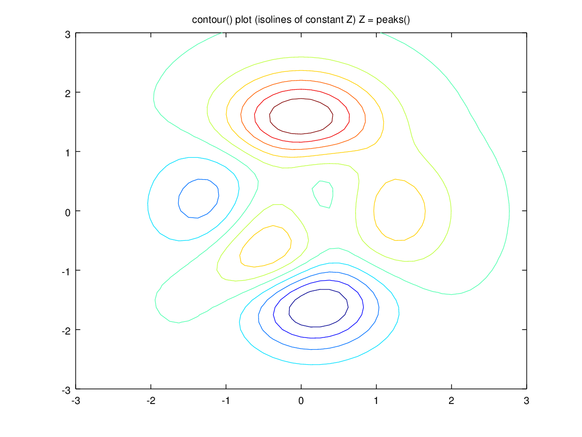
The following code
 clf;
 colormap ('default');
 [x, y, z] = peaks ();
 contour (x, y, z);
 title ({'contour() plot (isolines of constant Z)'; 'Z = peaks()'});
Produces the following figure
| Figure 1 |
|---|
 |
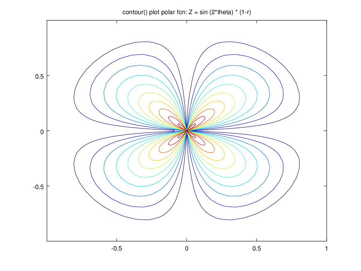
The following code
 clf;
 colormap ('default');
 [theta, r] = meshgrid (linspace (0,2*pi,64), linspace (0,1,64));
 [X, Y] = pol2cart (theta, r);
 Z = sin (2*theta) .* (1-r);
 contour (X, Y, abs (Z), 10);
 title ({'contour() plot'; 'polar fcn: Z = sin (2*theta) * (1-r)'});
Produces the following figure
| Figure 1 |
|---|
 |
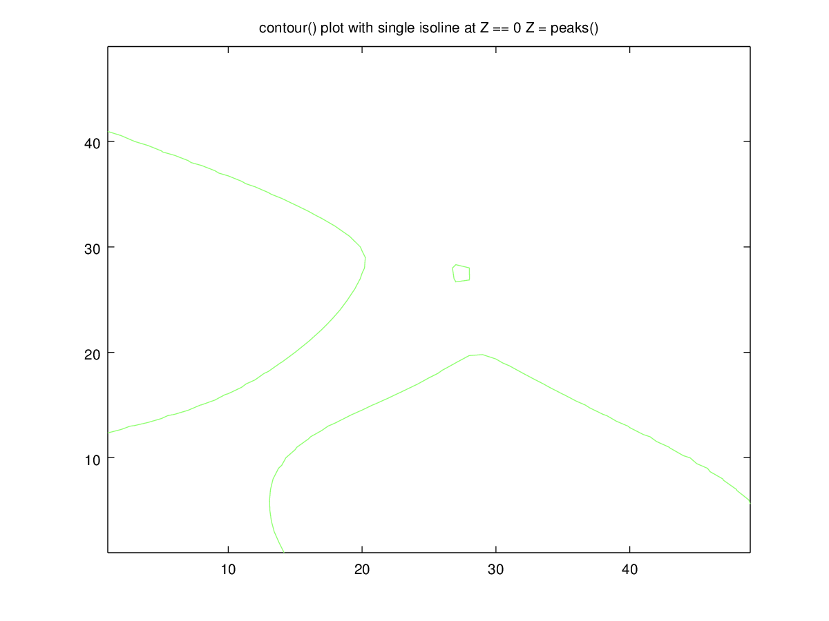
The following code
 clf;
 colormap ('default');
 z = peaks ();
 contour (z, [0 0]);
 title ({'contour() plot with single isoline at Z == 0'; 'Z = peaks()'});
Produces the following figure
| Figure 1 |
|---|
 |
Package: octave