
|
Octave-Forge - Extra packages for GNU Octave |
| Home · Packages · Developers · Documentation · FAQ · Bugs · Mailing Lists · Links · Code |
|
|
Octave-Forge - Extra packages for GNU Octave |
| Home · Packages · Developers · Documentation · FAQ · Bugs · Mailing Lists · Links · Code |
Toggle or set the "hold" state of the plotting engine which
determines whether new graphic objects are added to the plot or replace
the existing objects.
hold onRetain plot data and settings so that subsequent plot commands are displayed on a single graph.
hold allRetain plot line color, line style, data, and settings so that subsequent plot commands are displayed on a single graph with the next line color and style.
hold offRestore default graphics settings which clear the graph and reset axis properties before each new plot command. (default).
holdToggle the current hold state.
When given the additional argument hax, the hold state is modified
for this axis rather than the current axes returned by gca.
To query the current hold state use the ishold function.
See also: ishold, cla, clf, newplot.
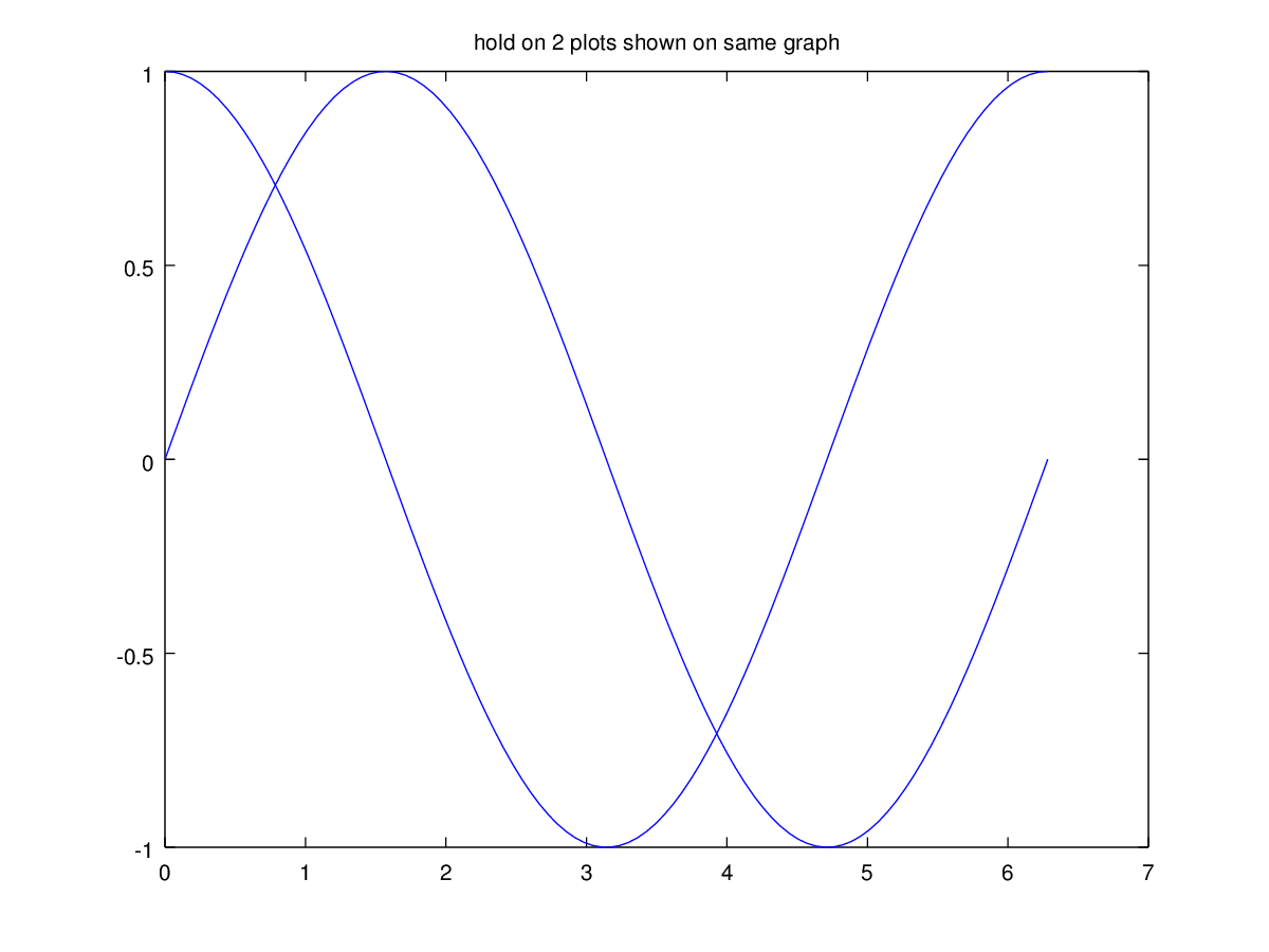
The following code
 clf;
 t = linspace (0, 2*pi, 100);
 plot (t, sin (t));
 hold on;
 plot (t, cos (t));
 title ({'hold on', '2 plots shown on same graph'});
 hold off;
Produces the following figure
| Figure 1 |
|---|
 |
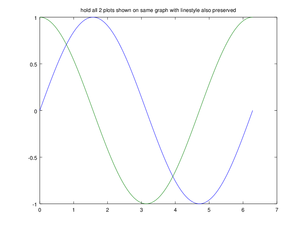
The following code
 clf;
 t = linspace (0, 2*pi, 100);
 plot (t, sin (t));
 hold all;
 plot (t, cos (t));
 title ({'hold all', '2 plots shown on same graph with linestyle also preserved'});
 hold off;
Produces the following figure
| Figure 1 |
|---|
 |
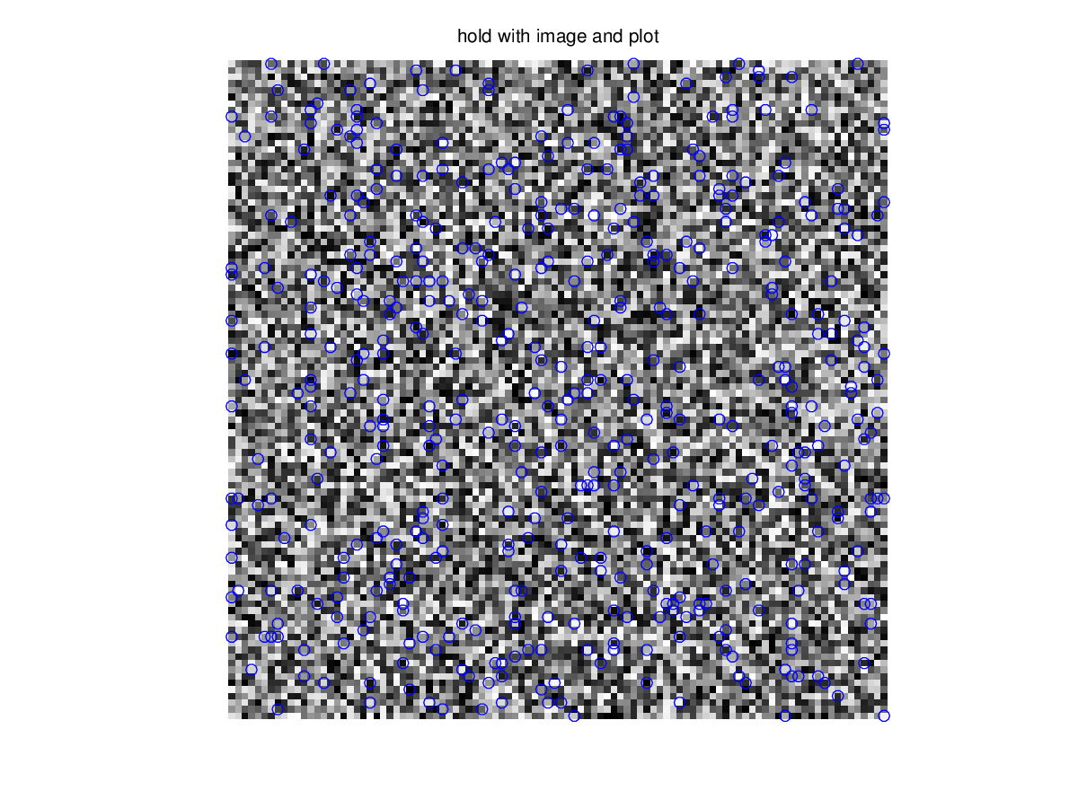
The following code
 clf;
 A = rand (100);
 [X, Y] = find (A > 0.95);
 imshow (A);
 hold on;
 plot (X, Y, 'o');
 hold off;
 title ('hold with image and plot');
Produces the following figure
| Figure 1 |
|---|
 |
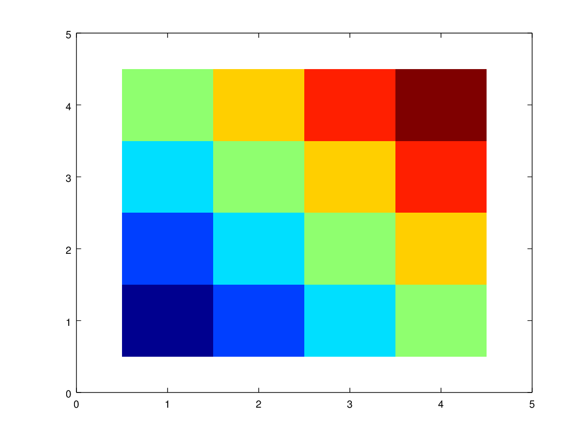
The following code
 clf;
 colormap ('default');
 hold on;
 imagesc (1 ./ hilb (4));
 plot (1:4, '-s');
 hold off;
Produces the following figure
| Figure 1 |
|---|
 |
The following code
 clf;
 colormap ('default');
 hold on;
 imagesc (1 ./ hilb (2));
 imagesc (1 ./ hilb (4));
 hold off;
Produces the following figure
| Figure 1 |
|---|
 |
The following code
 clf;
 colormap ('default');
 hold on;
 plot (1:4, '-s');
 imagesc (1 ./ hilb (4));
 hold off;
Produces the following figure
| Figure 1 |
|---|
 |
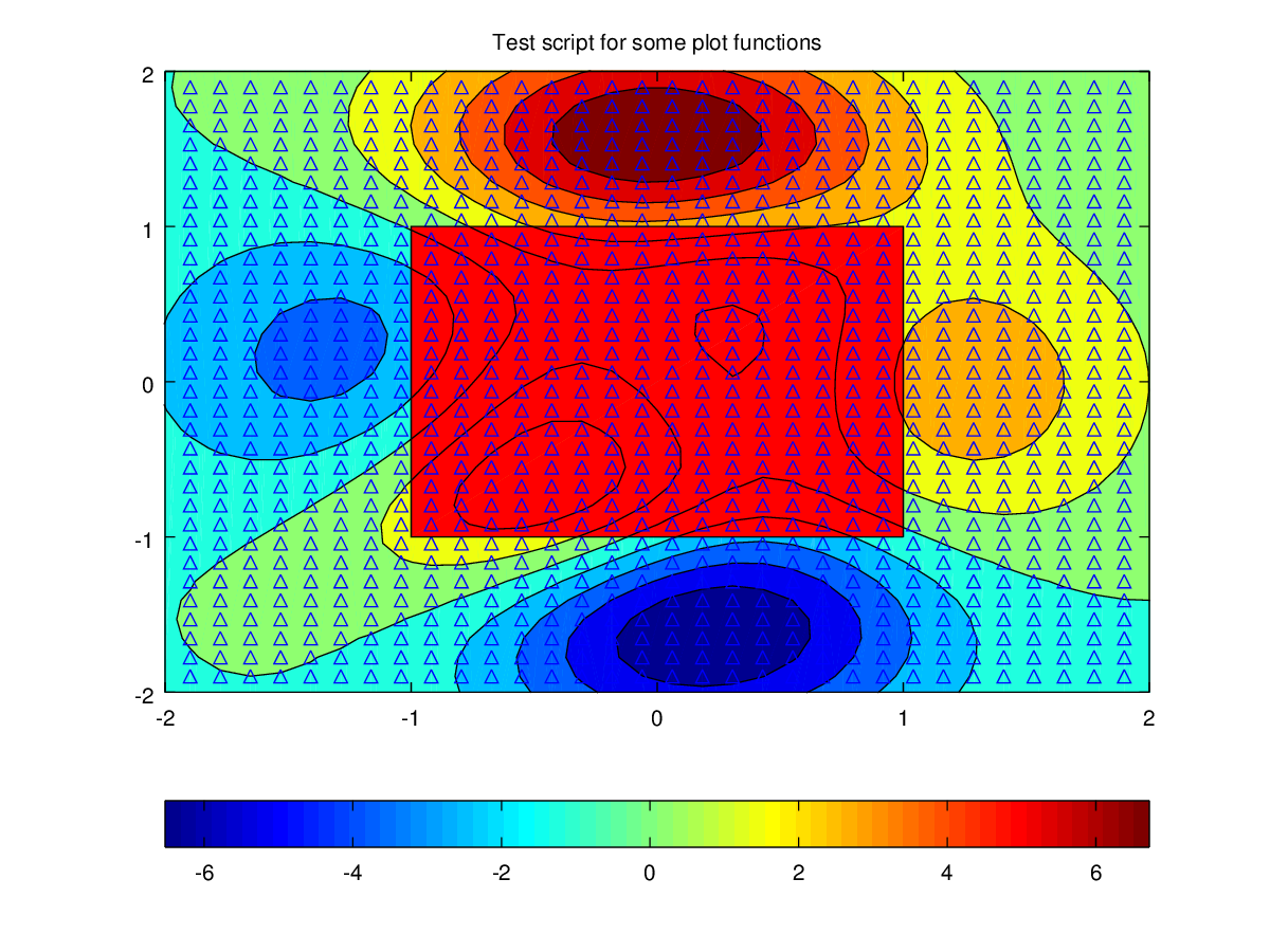
The following code
 clf;
 colormap ('default');
 t = linspace (-3, 3, 50);
 [x, y] = meshgrid (t, t);
 z = peaks (x, y);
 contourf (x, y, z, 10);
 hold on;
 plot (x(:), y(:), '^');
 patch ([-1.0 1.0 1.0 -1.0 -1.0], [-1.0 -1.0 1.0 1.0 -1.0], 'red');
 xlim ([-2.0 2.0]);
 ylim ([-2.0 2.0]);
 colorbar ('SouthOutside');
 title ('Test script for some plot functions');
Produces the following figure
| Figure 1 |
|---|
 |
Package: octave