
|
Octave-Forge - Extra packages for GNU Octave |
| Home · Packages · Developers · Documentation · FAQ · Bugs · Mailing Lists · Links · Code |
|
|
Octave-Forge - Extra packages for GNU Octave |
| Home · Packages · Developers · Documentation · FAQ · Bugs · Mailing Lists · Links · Code |
Display a scaled version of the matrix img as a color image.
The colormap is scaled so that the entries of the matrix occupy the entire
colormap. If climits = [lo, hi] is given, then
that range is set to the "clim" of the current axes.
The axis values corresponding to the matrix elements are specified in x and y, either as pairs giving the minimum and maximum values for the respective axes, or as values for each row and column of the matrix img.
The optional return value h is a graphics handle to the image.
Calling Forms: The imagesc function can be called in two forms:
High-Level and Low-Level. When invoked with normal options, the High-Level
form is used which first calls newplot to prepare the graphic figure
and axes. When the only inputs to image are property/value pairs
the Low-Level form is used which creates a new instance of an image object
and inserts it in the current axes.
See also: image, imshow, caxis.
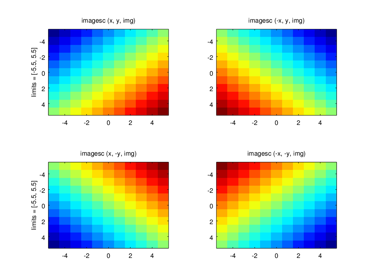
The following code
 clf;
 colormap ("default");
 img = 1 ./ hilb (11);
 x = y = -5:5;
 subplot (2,2,1);
  h = imagesc (x, y, img);
  ylabel ("limits = [-5.5, 5.5]");
  title ("imagesc (x, y, img)");
 subplot (2,2,2);
  h = imagesc (-x, y, img);
  title ("imagesc (-x, y, img)");
 subplot (2,2,3);
  h = imagesc (x, -y, img);
  title ("imagesc (x, -y, img)");
  ylabel ("limits = [-5.5, 5.5]");
 subplot (2,2,4);
  h = imagesc (-x, -y, img);
  title ("imagesc (-x, -y, img)");
Produces the following figure
| Figure 1 |
|---|
 |
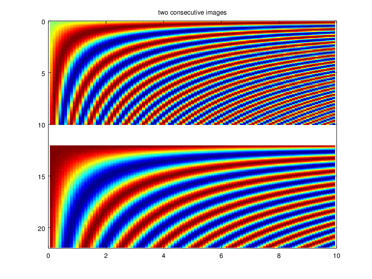
The following code
 clf;
 colormap ("default");
 g = 0.1:0.1:10;
 h = g'*g;
 imagesc (g, g, sin (h));
 hold on;
 imagesc (g, g+12, cos (h/2));
 axis ([0 10 0 22]);
 hold off;
 title ("two consecutive images");
Produces the following figure
| Figure 1 |
|---|
 |
The following code
 clf;
 colormap ("default");
 g = 0.1:0.1:10;
 h = g'*g;
 imagesc (g, g, sin (h));
 hold all;
 plot (g, 11.0 * ones (size (g)));
 imagesc (g, g+12, cos (h/2));
 axis ([0 10 0 22]);
 hold off;
 title ("image, line, image");
Produces the following figure
| Figure 1 |
|---|
 |
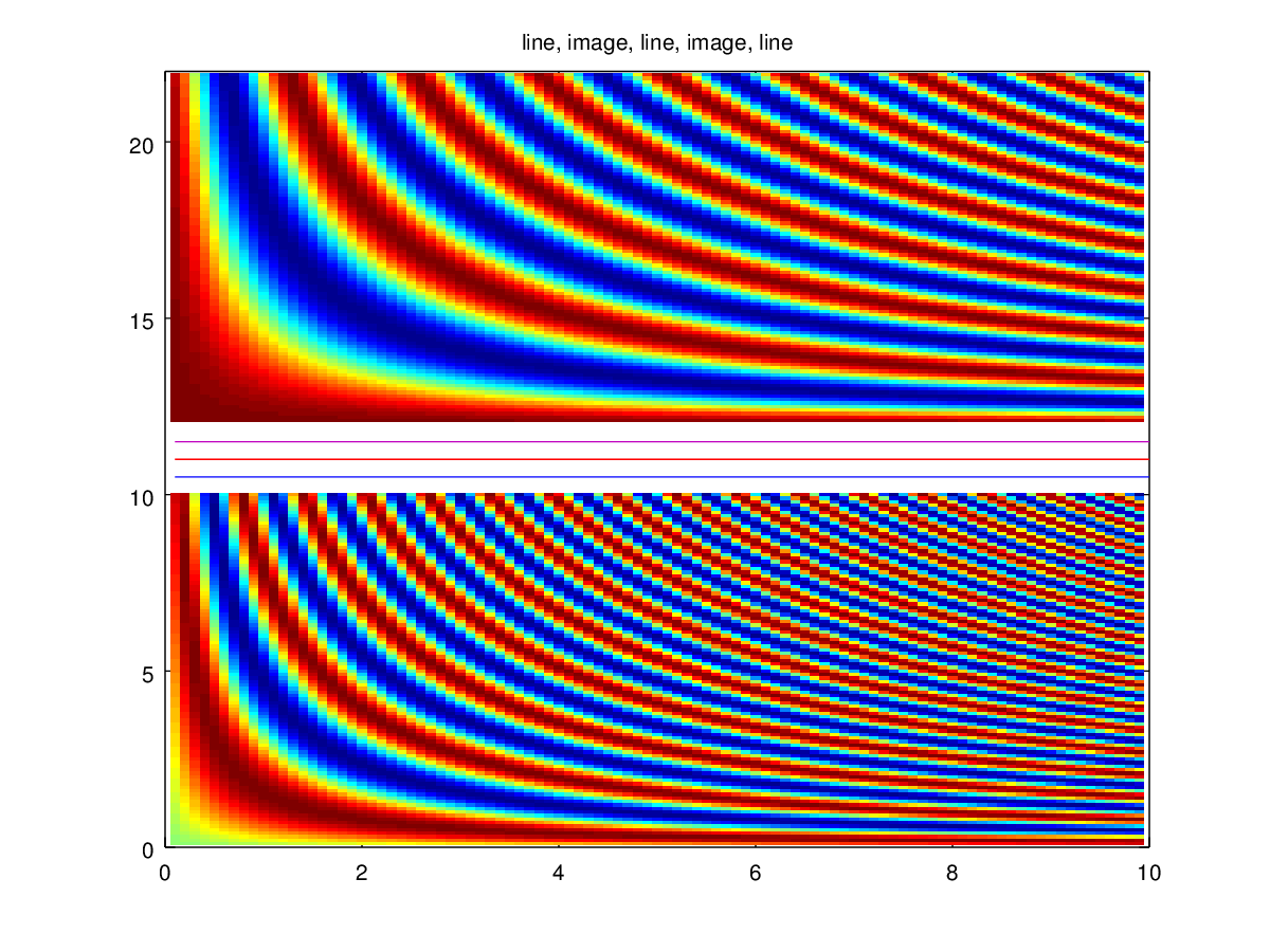
The following code
 clf;
 colormap ("default");
 g = 0.1:0.1:10;
 h = g'*g;
 plot (g, 10.5 * ones (size (g)));
 hold all;
 imagesc (g, g, sin (h));
 plot (g, 11.0 * ones (size (g)));
 imagesc (g, g+12, cos (h/2));
 plot (g, 11.5 * ones (size (g)));
 axis ([0 10 0 22]);
 hold off;
 title ("line, image, line, image, line");
Produces the following figure
| Figure 1 |
|---|
 |
Package: octave