
|
Octave-Forge - Extra packages for GNU Octave |
| Home · Packages · Developers · Documentation · FAQ · Bugs · Mailing Lists · Links · Code |
|
|
Octave-Forge - Extra packages for GNU Octave |
| Home · Packages · Developers · Documentation · FAQ · Bugs · Mailing Lists · Links · Code |
Calculate isosurface of 3-D data.
If called with one output argument and the first input argument
val is a three-dimensional array that contains the data of an
isosurface geometry and the second input argument iso keeps the
isovalue as a scalar value then return a structure array fv
that contains the fields Faces and Vertices at computed
points [x, y, z] = meshgrid (1:l, 1:m, 1:n). The output
argument fv can directly be taken as an input argument for the
patch function.
If called with further input arguments x, y and z which are three–dimensional arrays with the same size than val then the volume data is taken at those given points.
The string input argument "noshare" is only for compatibility and
has no effect. If given the string input argument
"verbose" then print messages to the command line interface about the
current progress.
If called with the input argument col which is a three-dimensional array of the same size than val then take those values for the interpolation of coloring the isosurface geometry. Add the field FaceVertexCData to the structure array fv.
If called with two or three output arguments then return the information about the faces f, vertices v and color data c as separate arrays instead of a single structure array.
If called with no output argument then directly process the
isosurface geometry with the patch command.
For example,
[x, y, z] = meshgrid (1:5, 1:5, 1:5);
val = rand (5, 5, 5);
isosurface (x, y, z, val, .5);
will directly draw a random isosurface geometry in a graphics window. Another example for an isosurface geometry with different additional coloring
N = 15;    # Increase number of vertices in each direction
iso = .4;  # Change isovalue to .1 to display a sphere
lin = linspace (0, 2, N);
[x, y, z] = meshgrid (lin, lin, lin);
c = abs ((x-.5).^2 + (y-.5).^2 + (z-.5).^2);
figure (); # Open another figure window

subplot (2,2,1); view (-38, 20);
[f, v] = isosurface (x, y, z, c, iso);
p = patch ("Faces", f, "Vertices", v, "EdgeColor", "none");
set (gca, "PlotBoxAspectRatioMode", "manual", ...
          "PlotBoxAspectRatio", [1 1 1]);
# set (p, "FaceColor", "green", "FaceLighting", "phong");
# light ("Position", [1 1 5]); # Available with the JHandles package

subplot (2,2,2); view (-38, 20);
p = patch ("Faces", f, "Vertices", v, "EdgeColor", "blue");
set (gca, "PlotBoxAspectRatioMode", "manual", ...
          "PlotBoxAspectRatio", [1 1 1]);
# set (p, "FaceColor", "none", "FaceLighting", "phong");
# light ("Position", [1 1 5]);

subplot (2,2,3); view (-38, 20);
[f, v, c] = isosurface (x, y, z, c, iso, y);
p = patch ("Faces", f, "Vertices", v, "FaceVertexCData", c, ...
           "FaceColor", "interp", "EdgeColor", "none");
set (gca, "PlotBoxAspectRatioMode", "manual", ...
          "PlotBoxAspectRatio", [1 1 1]);
# set (p, "FaceLighting", "phong");
# light ("Position", [1 1 5]);

subplot (2,2,4); view (-38, 20);
p = patch ("Faces", f, "Vertices", v, "FaceVertexCData", c, ...
           "FaceColor", "interp", "EdgeColor", "blue");
set (gca, "PlotBoxAspectRatioMode", "manual", ...
          "PlotBoxAspectRatio", [1 1 1]);
# set (p, "FaceLighting", "phong");
# light ("Position", [1 1 5]);
See also: isonormals, isocolors.
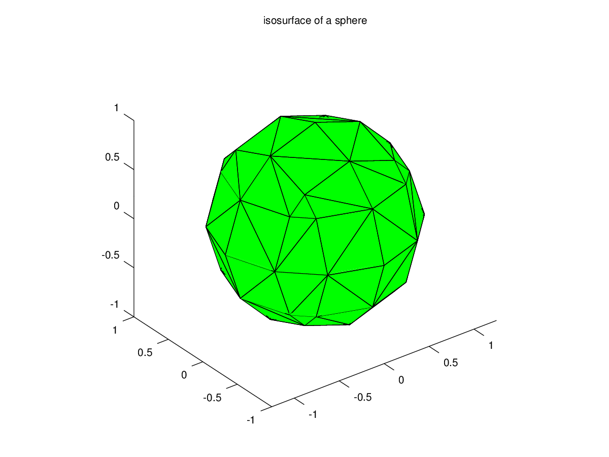
The following code
 clf;
 [x,y,z] = meshgrid (-2:0.5:2, -2:0.5:2, -2:0.5:2);
 v = x.^2 + y.^2 + z.^2;
 isosurface (x, y, z, v, 1);
 axis equal;
 title ('isosurface of a sphere');
Produces the following figure
| Figure 1 |
|---|
 |
Package: octave