
|
Octave-Forge - Extra packages for GNU Octave |
| Home · Packages · Developers · Documentation · FAQ · Bugs · Mailing Lists · Links · Code |
|
|
Octave-Forge - Extra packages for GNU Octave |
| Home · Packages · Developers · Documentation · FAQ · Bugs · Mailing Lists · Links · Code |
Create patch object in the current axes with vertices at locations (x, y) and of color c.
If the vertices are matrices of size MxN then each polygon patch has M vertices and a total of N polygons will be created. If some polygons do not have M vertices use NaN to represent "no vertex". If the z input is present then 3-D patches will be created.
The color argument c can take many forms. To create polygons
which all share a single color use a string value (e.g., "r" for
red), a scalar value which is scaled by caxis and indexed into the
current colormap, or a 3-element RGB vector with the precise TrueColor.
If c is a vector of length N then the ith polygon will have a color
determined by scaling entry c(i) according to caxis and then
indexing into the current colormap. More complicated coloring situations
require directly manipulating patch property/value pairs.
Instead of specifying polygons by matrices x and y, it is
possible to present a unique list of vertices and then a list of polygon
faces created from those vertices. In this case the
"Vertices" matrix will be an Nx2 (2-D patch) or
Nx3 (3-D path). The MxN "Faces" matrix
describes M polygons having N vertices—each row describes a
single polygon and each column entry is an index into the
"Vertices" matrix to identify a vertex. The patch object
can be created by directly passing the property/value pairs
"Vertices"/verts, "Faces"/faces as
inputs.
A third input form is to create a structure fv with the fields
"vertices", "faces", and optionally
"facevertexcdata".
If the first argument hax is an axes handle, then plot into this axis,
rather than the current axes returned by gca.
The optional return value h is a graphics handle to the created patch object.
Implementation Note: Patches are highly configurable objects. To truly
customize them requires setting patch properties directly. Useful patch
properties are: "cdata", "edgecolor",
"facecolor", "faces", "facevertexcdata".
See also: fill, get, set.
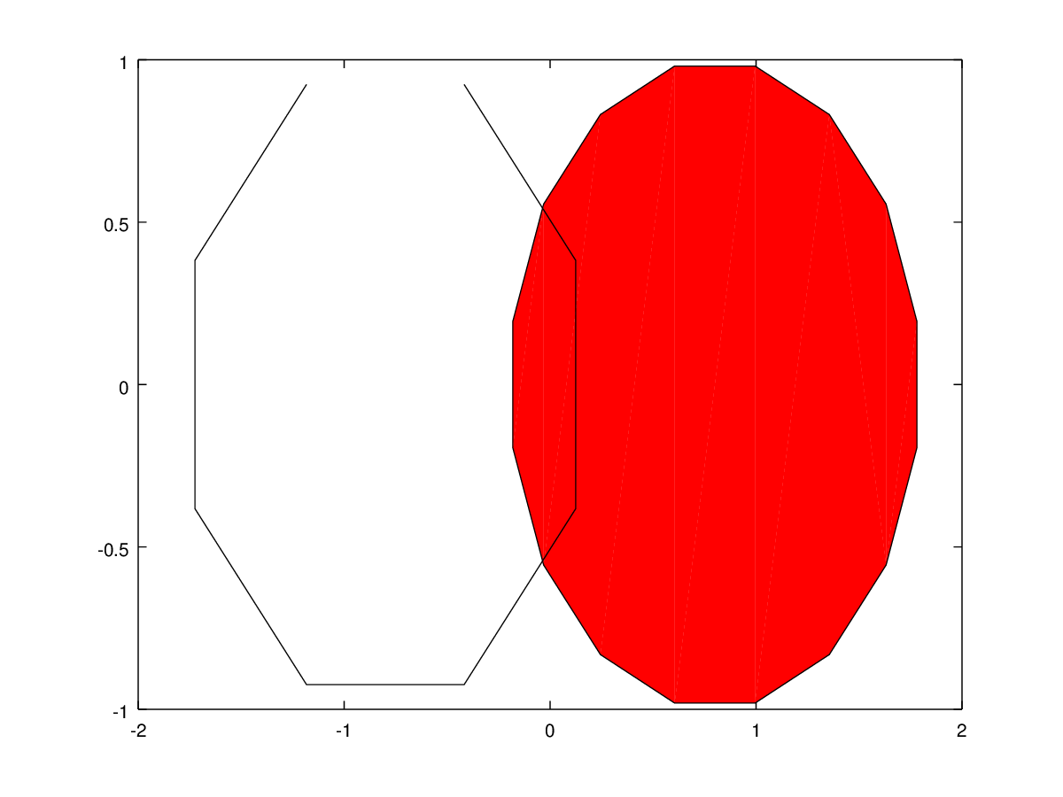
The following code
 %% Patches with same number of vertices
 clf;
 t1 = (1/16:1/8:1)' * 2*pi;
 t2 = ((1/16:1/8:1)' + 1/32) * 2*pi;
 x1 = sin (t1) - 0.8;
 y1 = cos (t1);
 x2 = sin (t2) + 0.8;
 y2 = cos (t2);
 patch ([x1,x2], [y1,y2], 'r');
Produces the following figure
| Figure 1 |
|---|
 |
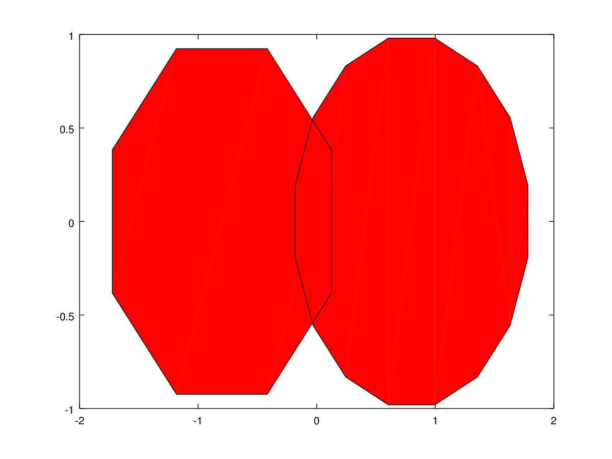
The following code
 %% Unclosed patch
 clf;
 t1 = (1/16:1/8:1)' * 2*pi;
 t2 = ((1/16:1/16:1)' + 1/32) * 2*pi;
 x1 = sin (t1) - 0.8;
 y1 = cos (t1);
 x2 = sin (t2) + 0.8;
 y2 = cos (t2);
 patch ([[x1;NaN(8,1)],x2], [[y1;NaN(8,1)],y2], 'r');
Produces the following figure
| Figure 1 |
|---|
 |
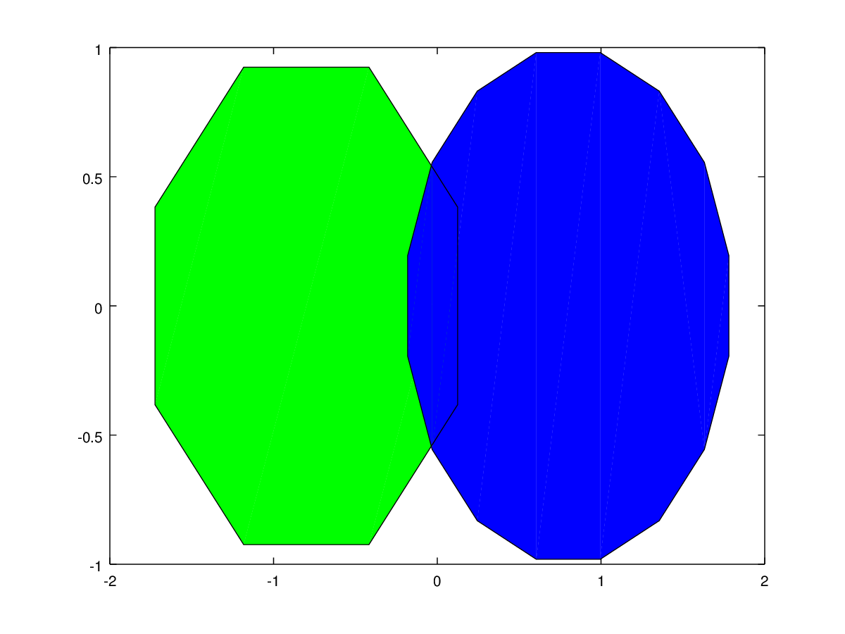
The following code
 %% Specify vertices and faces separately
 clf;
 t1 = (1/16:1/8:1)' * 2*pi;
 t2 = ((1/16:1/16:1)' + 1/32) * 2*pi;
 x1 = sin (t1) - 0.8;
 y1 = cos (t1);
 x2 = sin (t2) + 0.8;
 y2 = cos (t2);
 vert = [x1, y1; x2, y2];
 fac = [1:8,NaN(1,8);9:24];
 patch ('Faces',fac, 'Vertices',vert, 'FaceColor','r');
Produces the following figure
| Figure 1 |
|---|
 |
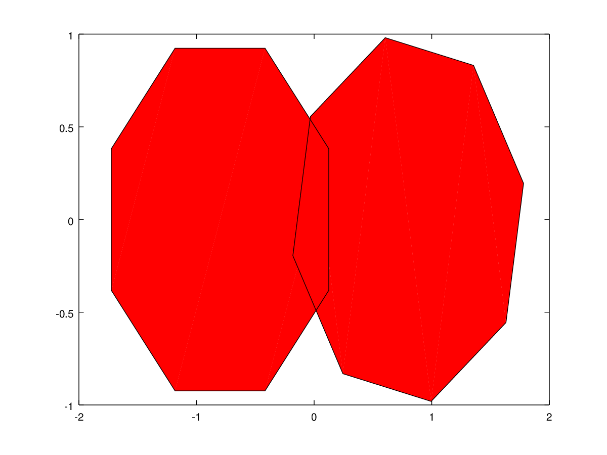
The following code
 %% Specify vertices and faces separately
 clf;
 t1 = (1/16:1/8:1)' * 2*pi;
 t2 = ((1/16:1/16:1)' + 1/32) * 2*pi;
 x1 = sin (t1) - 0.8;
 y1 = cos (t1);
 x2 = sin (t2) + 0.8;
 y2 = cos (t2);
 vert = [x1, y1; x2, y2];
 fac = [1:8,NaN(1,8);9:24];
 patch ('Faces',fac, 'Vertices',vert, ...
        'FaceVertexCData',[0, 1, 0; 0, 0, 1], 'FaceColor', 'flat');
Produces the following figure
| Figure 1 |
|---|
 |
The following code
 %% Property change on multiple patches
 clf;
 t1 = (1/16:1/8:1)' * 2*pi;
 t2 = ((1/16:1/8:1)' + 1/32) * 2*pi;
 x1 = sin (t1) - 0.8;
 y1 = cos (t1);
 x2 = sin (t2) + 0.8;
 y2 = cos (t2);
 h = patch ([x1,x2], [y1,y2], cat (3, [0,0],[1,0],[0,1]));
 pause (1);
 set (h, 'FaceColor', 'r');
Produces the following figure
| Figure 1 |
|---|
 |
The following code
 clf;
 vertices = [0, 0, 0;
             1, 0, 0;
             1, 1, 0;
             0, 1, 0;
             0.5, 0.5, 1];
 faces = [1, 2, 5;
          2, 3, 5;
          3, 4, 5;
          4, 1, 5];
 patch ('Vertices', vertices, 'Faces', faces, ...
        'FaceVertexCData', jet (4), 'FaceColor', 'flat');
 view (-37.5, 30);
Produces the following figure
| Figure 1 |
|---|
 |
The following code
 clf;
 vertices = [0, 0, 0;
             1, 0, 0;
             1, 1, 0;
             0, 1, 0;
             0.5, 0.5, 1];
 faces = [1, 2, 5;
          2, 3, 5;
          3, 4, 5;
          4, 1, 5];
 patch  ('Vertices', vertices, 'Faces', faces, ...
        'FaceVertexCData', jet (5), 'FaceColor', 'interp');
 view (-37.5, 30);
Produces the following figure
| Figure 1 |
|---|
 |
The following code
 clf;
 colormap (jet (64));
 x = [0 1 1 0];
 y = [0 0 1 1];
 subplot (2,1,1);
  title ('Blue, Light-Green, and Red Horizontal Bars');
  patch (x, y + 0, 1);
  patch (x, y + 1, 2);
  patch (x, y + 2, 3);
 subplot (2,1,2);
  title ('Blue, Light-Green, and Red Vertical Bars');
  patch (x + 0, y, 1 * ones (size (x)));
  patch (x + 1, y, 2 * ones (size (x)));
  patch (x + 2, y, 3 * ones (size (x)));
Produces the following figure
| Figure 1 |
|---|
 |
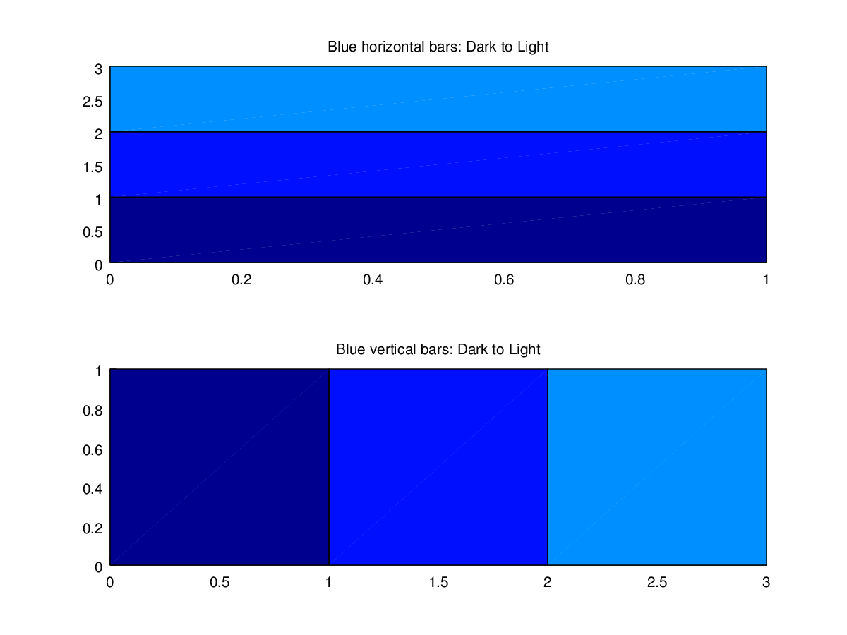
The following code
 clf;
 colormap (jet (64));
 x = [0 1 1 0];
 y = [0 0 1 1];
 subplot (2,1,1);
  title ('Blue horizontal bars: Dark to Light');
  patch (x, y + 0, 1, 'cdatamapping', 'direct');
  patch (x, y + 1, 9, 'cdatamapping', 'direct');
  patch (x, y + 2, 17, 'cdatamapping', 'direct');
 subplot (2,1,2);
  title ('Blue vertical bars: Dark to Light');
  patch (x + 0, y, 1 * ones (size (x)), 'cdatamapping', 'direct');
  patch (x + 1, y, 9 * ones (size (x)), 'cdatamapping', 'direct');
  patch (x + 2, y, 17 * ones (size (x)), 'cdatamapping', 'direct');
Produces the following figure
| Figure 1 |
|---|
 |
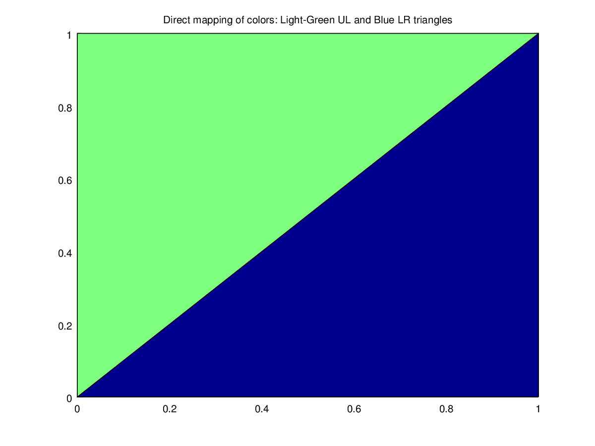
The following code
 clf;
 colormap (jet (64));
 x = [ 0 0; 1 1; 1 0 ];
 y = [ 0 0; 0 1; 1 1 ];
 p = patch (x, y, 'b');
 set (p, 'cdatamapping', 'direct', 'facecolor', 'flat', 'cdata', [1 32]);
 title ('Direct mapping of colors: Light-Green UL and Blue LR triangles');
Produces the following figure
| Figure 1 |
|---|
 |
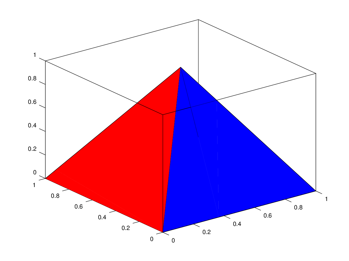
The following code
 clf;
 colormap (jet (64));
 x = [ 0 0; 1 1; 1 0 ];
 y = [ 0 0; 0 1; 1 1 ];
 p = patch (x, y, [1 32]);
 title ('Autoscaling of colors: Red UL and Blue LR triangles');
Produces the following figure
| Figure 1 |
|---|
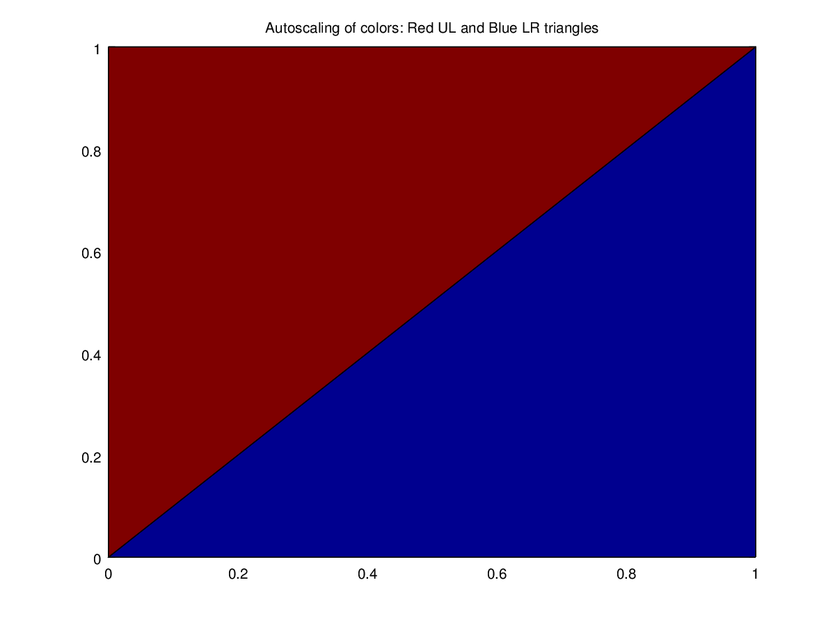 |
Package: octave