
|
Octave-Forge - Extra packages for GNU Octave |
| Home · Packages · Developers · Documentation · FAQ · Bugs · Mailing Lists · Links · Code |
|
|
Octave-Forge - Extra packages for GNU Octave |
| Home · Packages · Developers · Documentation · FAQ · Bugs · Mailing Lists · Links · Code |
Draw a 2-D scatter plot.
A marker is plotted at each point defined by the coordinates in the vectors x and y.
The size of the markers is determined by s, which can be a scalar or a vector of the same length as x and y. If s is not given, or is an empty matrix, then a default value of 8 points is used.
The color of the markers is determined by c, which can be a string defining a fixed color; a 3-element vector giving the red, green, and blue components of the color; a vector of the same length as x that gives a scaled index into the current colormap; or an Nx3 matrix defining the RGB color of each marker individually.
The marker to use can be changed with the style argument, that is a
string defining a marker in the same manner as the plot command.
If no marker is specified it defaults to "o" or circles.
If the argument "filled" is given then the markers are filled.
Additional property/value pairs are passed directly to the underlying patch object.
If the first argument hax is an axes handle, then plot into this axis,
rather than the current axes returned by gca.
The optional return value h is a graphics handle to the created patch object.
Example:
x = randn (100, 1);
y = randn (100, 1);
scatter (x, y, [], sqrt (x.^2 + y.^2));
See also: scatter3, patch, plot.
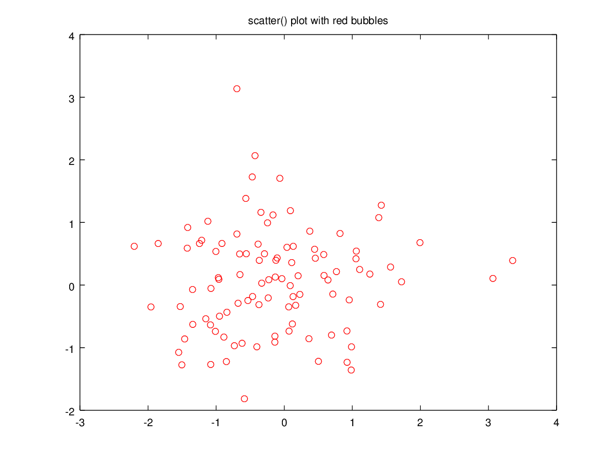
The following code
 clf;
 x = randn (100, 1);
 y = randn (100, 1);
 scatter (x, y, 'r');
 title ('scatter() plot with red bubbles');
Produces the following figure
| Figure 1 |
|---|
 |
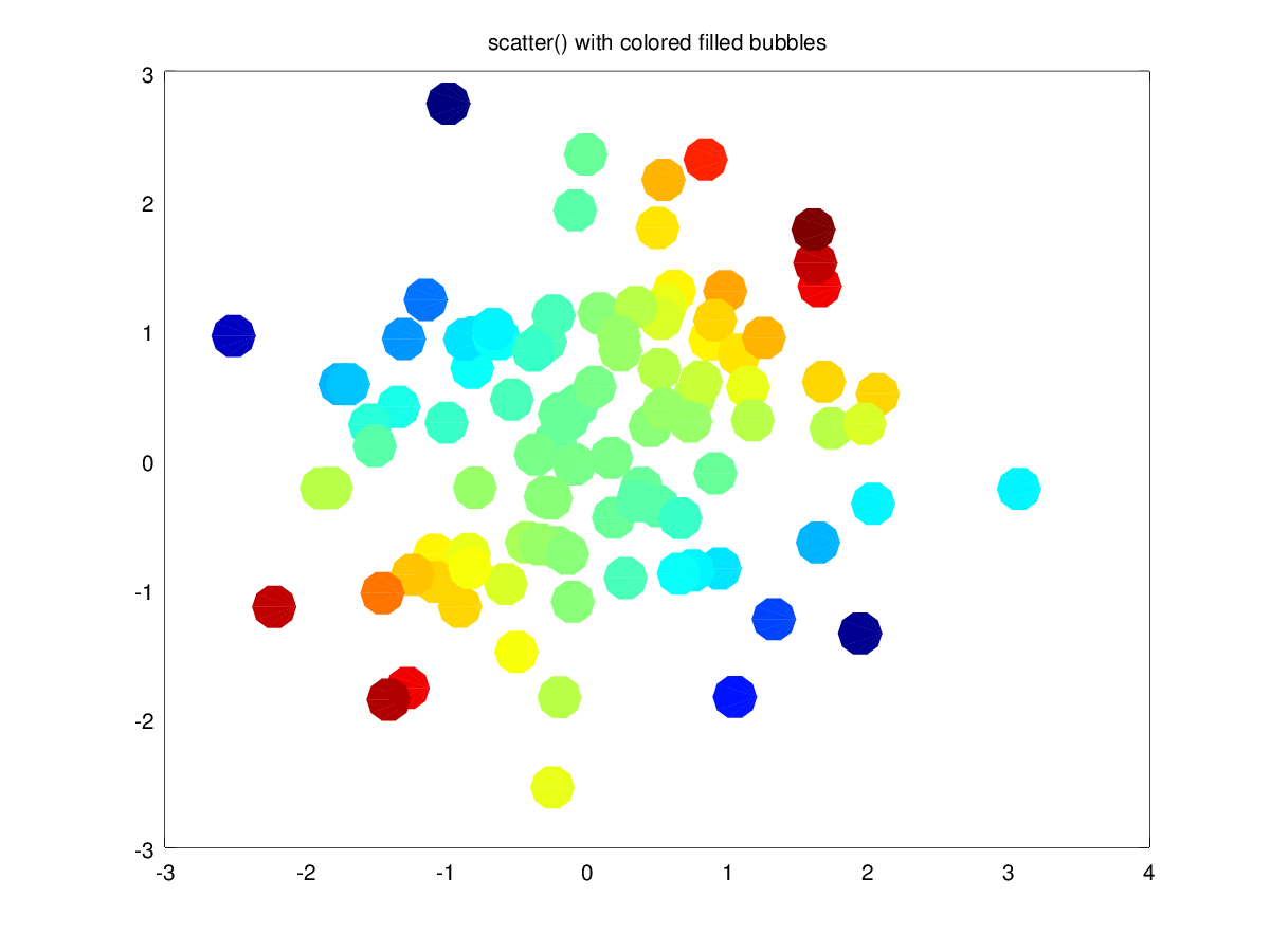
The following code
 clf;
 x = randn (100, 1);
 y = randn (100, 1);
 c = x .* y;
 scatter (x, y, 20, c, 'filled');
 title ('scatter() with colored filled bubbles');
Produces the following figure
| Figure 1 |
|---|
 |
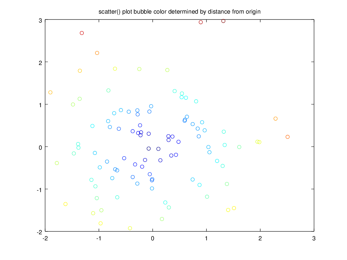
The following code
 clf;
 x = randn (100, 1);
 y = randn (100, 1);
 scatter (x, y, [], sqrt (x.^2 + y.^2));
 title ({'scatter() plot'; ...
         'bubble color determined by distance from origin'});
Produces the following figure
| Figure 1 |
|---|
 |
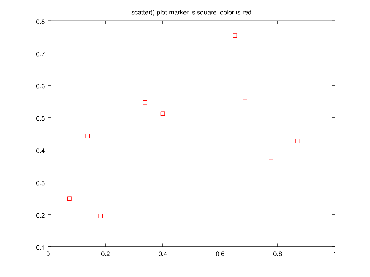
The following code
 clf;
 rand_10x1_data5 = [0.777753, 0.093848, 0.183162, 0.399499, 0.337997, 0.686724, 0.073906, 0.651808, 0.869273, 0.137949];
 rand_10x1_data6 = [0.37460, 0.25027, 0.19510, 0.51182, 0.54704, 0.56087, 0.24853, 0.75443, 0.42712, 0.44273];
 x = rand_10x1_data5;
 y = rand_10x1_data6;
 s = 10 - 10*log (x.^2 + y.^2);
 h = scatter (x, y, [], 'r', 's');
 title ({'scatter() plot'; ...
         'marker is square, color is red'});
Produces the following figure
| Figure 1 |
|---|
 |
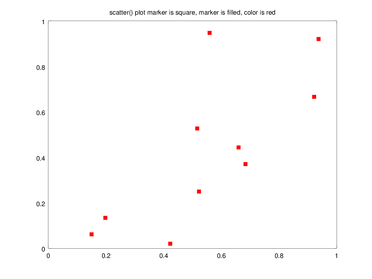
The following code
 clf;
 rand_10x1_data3 = [0.42262, 0.51623, 0.65992, 0.14999, 0.68385, 0.55929, 0.52251, 0.92204, 0.19762, 0.93726];
 rand_10x1_data4 = [0.020207, 0.527193, 0.443472, 0.061683, 0.370277, 0.947349, 0.249591, 0.666304, 0.134247, 0.920356];
 x = rand_10x1_data3;
 y = rand_10x1_data4;
 s = 10 - 10*log (x.^2 + y.^2);
 h = scatter (x, y, [], 'r', 's', 'filled');
 title ({'scatter() plot'; ...
         'marker is square, marker is filled, color is red'});
Produces the following figure
| Figure 1 |
|---|
 |
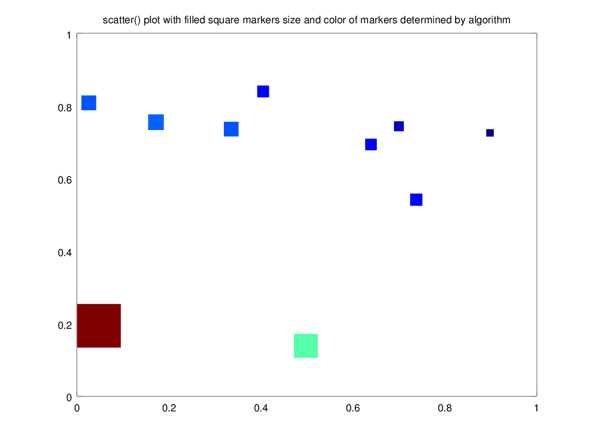
The following code
 clf;
 rand_10x1_data1 = [0.171577, 0.404796, 0.025469, 0.335309, 0.047814, 0.898480, 0.639599, 0.700247, 0.497798, 0.737940];
 rand_10x1_data2 = [0.75495, 0.83991, 0.80850, 0.73603, 0.19360, 0.72573, 0.69371, 0.74388, 0.13837, 0.54143];
 x = rand_10x1_data1;
 y = rand_10x1_data2;
 s = 10 - 10*log (x.^2 + y.^2);
 h = scatter (x, y, s, s, 's', 'filled');
 title ({'scatter() plot with filled square markers', ...
         'size and color of markers determined by algorithm'});
Produces the following figure
| Figure 1 |
|---|
 |
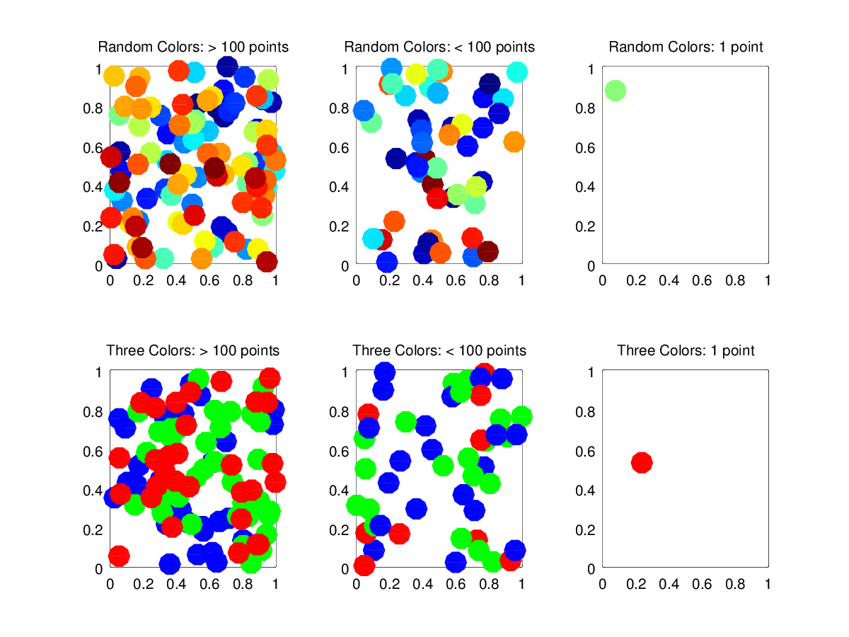
The following code
 clf;
 k = 1;
 for m = [1, 3]
   for n = [101, 50, 1]
     x = rand (n, 1);
     y = rand (n, 1);
     if (m > 1)
       str = 'Three Colors';
       idx = ceil (rand (n, 1) * 3);
       colors = eye (3);
       colors = colors(idx, :);
     else
       str = 'Random Colors';
       colors = rand (n, m);
     end
     if (n == 1)
       str = sprintf ('%s: 1 point', str);
     elseif (n < 100)
       str = sprintf ('%s: < 100 points', str);
     else
       str = sprintf ('%s: > 100 points', str);
     end
     subplot (2,3,k);
     k = k + 1;
     scatter (x, y, 15, colors, 'filled');
     axis ([0 1 0 1]);
     title (str);
   end
 end
Produces the following figure
| Figure 1 |
|---|
 |
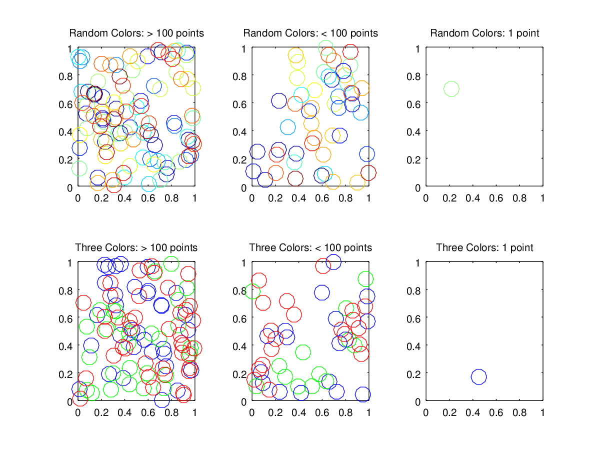
The following code
 clf;
 k = 1;
 for m = [1, 3]
   for n = [101, 50, 1]
     x = rand (n, 1);
     y = rand (n, 1);
     if (m > 1)
       str = 'Three Colors';
       idx = ceil (rand (n, 1) * 3);
       colors = eye (3);
       colors = colors(idx, :);
     else
       str = 'Random Colors';
       colors = rand (n, m);
     end
     if (n == 1)
       str = sprintf ('%s: 1 point', str);
     elseif (n < 100)
       str = sprintf ('%s: < 100 points', str);
     else
       str = sprintf ('%s: > 100 points', str);
     end
     subplot (2,3,k);
     k = k + 1;
     scatter (x, y, 15, colors);
     axis ([0 1 0 1]);
     title (str);
   end
 end
Produces the following figure
| Figure 1 |
|---|
 |
Package: octave