
|
Octave-Forge - Extra packages for GNU Octave |
| Home · Packages · Developers · Documentation · FAQ · Bugs · Mailing Lists · Links · Code |
|
|
Octave-Forge - Extra packages for GNU Octave |
| Home · Packages · Developers · Documentation · FAQ · Bugs · Mailing Lists · Links · Code |
Determine the execution time of an expression (f) for various input values (n).
The n are log-spaced from 1 to max_n. For each n, an initialization expression (init) is computed to create any data needed for the test. If a second expression (f2) is given then the execution times of the two expressions are compared. When called without output arguments the results are printed to stdout and displayed graphically.
fThe code expression to evaluate.
max_nThe maximum test length to run. The default value is 100. Alternatively,
use [min_n, max_n] or specify the n exactly with
[n1, n2, …, nk].
initInitialization expression for function argument values. Use k for
the test number and n for the size of the test. This should compute
values for all variables used by f. Note that init will be
evaluated first for k = 0, so things which are constant throughout
the test series can be computed once. The default value is
x = randn (n, 1).
f2An alternative expression to evaluate, so that the speed of two
expressions can be directly compared. The default is [].
tolTolerance used to compare the results of expression f and expression
f2. If tol is positive, the tolerance is an absolute one.
If tol is negative, the tolerance is a relative one. The default is
eps. If tol is Inf, then no comparison will be made.
orderThe time complexity of the expression O(a*n^p). This is a
structure with fields a and p.
nThe values n for which the expression was calculated AND the execution time was greater than zero.
T_fThe nonzero execution times recorded for the expression f in seconds.
T_f2The nonzero execution times recorded for the expression f2 in seconds.
If required, the mean time ratio is simply mean (T_f ./ T_f2).
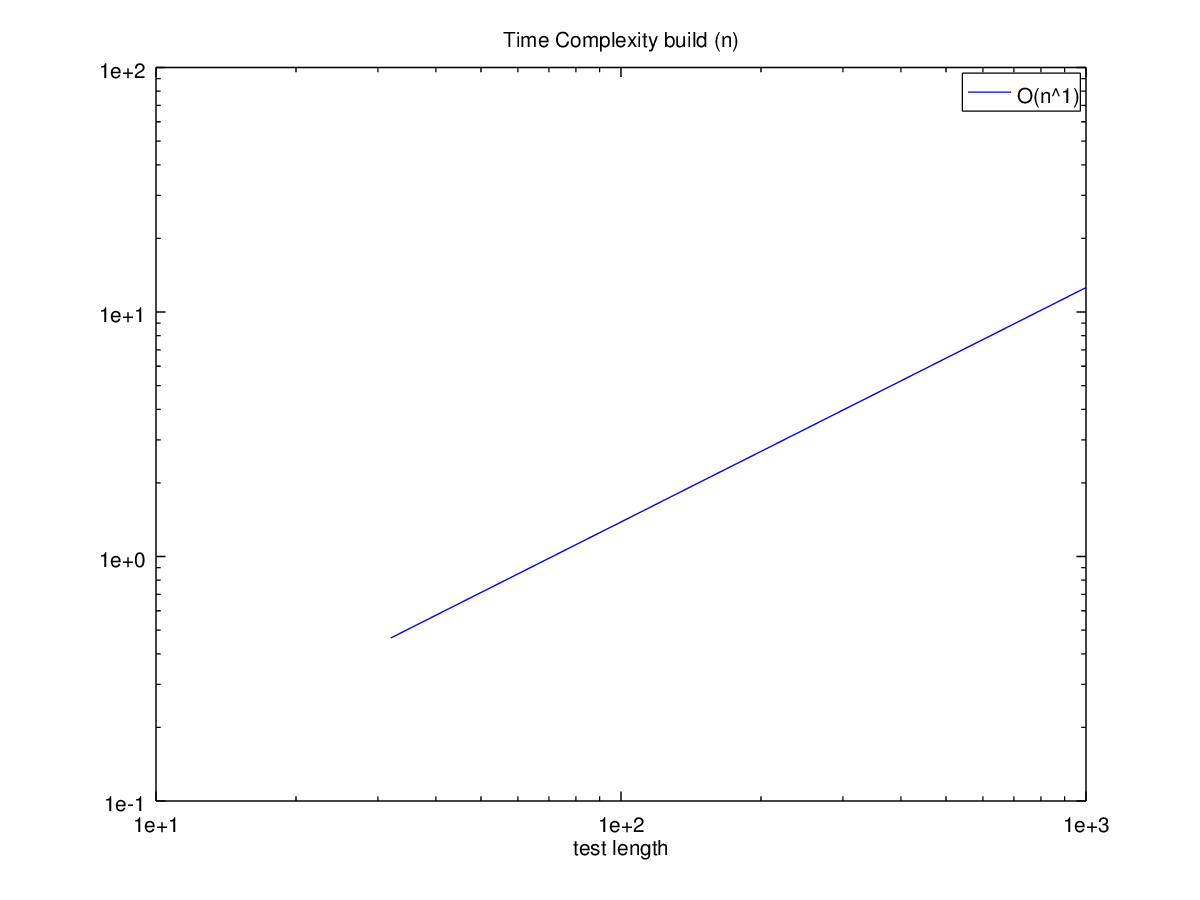
The slope of the execution time graph shows the approximate power of the asymptotic running time O(n^p). This power is plotted for the region over which it is approximated (the latter half of the graph). The estimated power is not very accurate, but should be sufficient to determine the general order of an algorithm. It should indicate if, for example, the implementation is unexpectedly O(n^2) rather than O(n) because it extends a vector each time through the loop rather than pre-allocating storage. In the current version of Octave, the following is not the expected O(n).
speed ("for i = 1:n, y{i} = x(i); endfor", "", [1000, 10000])
But it is if you preallocate the cell array y:
speed ("for i = 1:n, y{i} = x(i); endfor", ...
       "x = rand (n, 1); y = cell (size (x));", [1000, 10000])
An attempt is made to approximate the cost of individual operations, but
it is wildly inaccurate. You can improve the stability somewhat by doing
more work for each n. For example:
speed ("airy(x)", "x = rand (n, 10)", [10000, 100000])
When comparing two different expressions (f, f2), the slope of the line on the speedup ratio graph should be larger than 1 if the new expression is faster. Better algorithms have a shallow slope. Generally, vectorizing an algorithm will not change the slope of the execution time graph, but will shift it relative to the original. For example:
speed ("sum (x)", "", [10000, 100000], ...
       "v = 0; for i = 1:length (x), v += x(i); endfor")
The following is a more complex example. If there was an original version
of xcorr using for loops and a second version using an FFT, then
one could compare the run speed for various lags as follows, or for a fixed
lag with varying vector lengths as follows:
speed ("xcorr (x, n)", "x = rand (128, 1);", 100,
       "xcorr_orig (x, n)", -100*eps)
speed ("xcorr (x, 15)", "x = rand (20+n, 1);", 100,
       "xcorr_orig (x, n)", -100*eps)
Assuming one of the two versions is in xcorr_orig, this would compare their
speed and their output values. Note that the FFT version is not exact, so
one must specify an acceptable tolerance on the comparison 100*eps.
In this case, the comparison should be computed relatively, as
abs ((x - y) ./ y) rather than absolutely as
abs (x - y).
Type example ("speed") to see some real examples or demo ("speed") to run them.
The following code
 fstr_build_orig = cstrcat (
   "function x = build_orig (n)\n",
   "  ## extend the target vector on the fly\n",
   "  for i=0:n-1, x([1:100]+i*100) = 1:100; endfor\n",
   "endfunction");
 fstr_build = cstrcat (
   "function x = build (n)\n",
   "  ## preallocate the target vector\n",
   "  x = zeros (1, n*100);\n",
   "  for i=0:n-1, x([1:100]+i*100) = 1:100; endfor\n",
   "endfunction");

 disp ("-----------------------");
 disp (fstr_build_orig);
 disp ("-----------------------");
 disp (fstr_build);
 disp ("-----------------------");

 ## Eval functions strings to create them in the current context
 eval (fstr_build_orig);
 eval (fstr_build);

 disp ("Preallocated vector test.\nThis takes a little while...");
 speed ("build (n)", "", 1000, "build_orig (n)");
 clear -f build build_orig
 disp ("-----------------------");
 disp ("Note how much faster it is to pre-allocate a vector.");
 disp ("Notice the peak speedup ratio.");
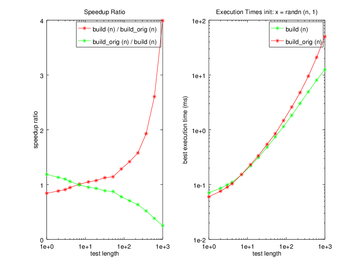
Produces the following output
-----------------------
function x = build_orig (n)
  ## extend the target vector on the fly
  for i=0:n-1, x([1:100]+i*100) = 1:100; endfor
endfunction
-----------------------
function x = build (n)
  ## preallocate the target vector
  x = zeros (1, n*100);
  for i=0:n-1, x([1:100]+i*100) = 1:100; endfor
endfunction
-----------------------
Preallocated vector test.
This takes a little while...
testing build (n)
init: x = randn (n, 1)
n1 = 1  n2 = 2  n3 = 3  n4 = 4  n5 = 7  n6 = 12  n7 = 19  n8 = 32  n9 = 52  n10 = 85  n11 = 139  n12 = 228  n13 = 373  n14 = 611  n15 = 1000

Mean runtime ratio = 1.45 for 'build_orig (n)' vs 'build (n)'

For build (n):
  asymptotic power: O(n^1)
  approximate time per operation: 10 us
-----------------------
Note how much faster it is to pre-allocate a vector.
Notice the peak speedup ratio.
and the following figures
| Figure 1 | Figure 2 |
|---|---|
 |
 |
The following code
 fstr_build_orig = cstrcat (
   "function x = build_orig (n)\n",
   "  for i=0:n-1, x([1:100]+i*100) = 1:100; endfor\n",
   "endfunction");
 fstr_build = cstrcat (
   "function x = build (n)\n",
   "  idx = [1:100]';\n",
   "  x = idx(:,ones(1,n));\n",
   "  x = reshape (x, 1, n*100);\n",
   "endfunction");

 disp ("-----------------------");
 disp (fstr_build_orig);
 disp ("-----------------------");
 disp (fstr_build);
 disp ("-----------------------");

 ## Eval functions strings to create them in the current context
 eval (fstr_build_orig);
 eval (fstr_build);

 disp ("Vectorized test.\nThis takes a little while...");
 speed ("build (n)", "", 1000, "build_orig (n)");
 clear -f build build_orig
 disp ("-----------------------");
 disp ("This time, the for loop is done away with entirely.");
 disp ("Notice how much bigger the speedup is than in example 1.");
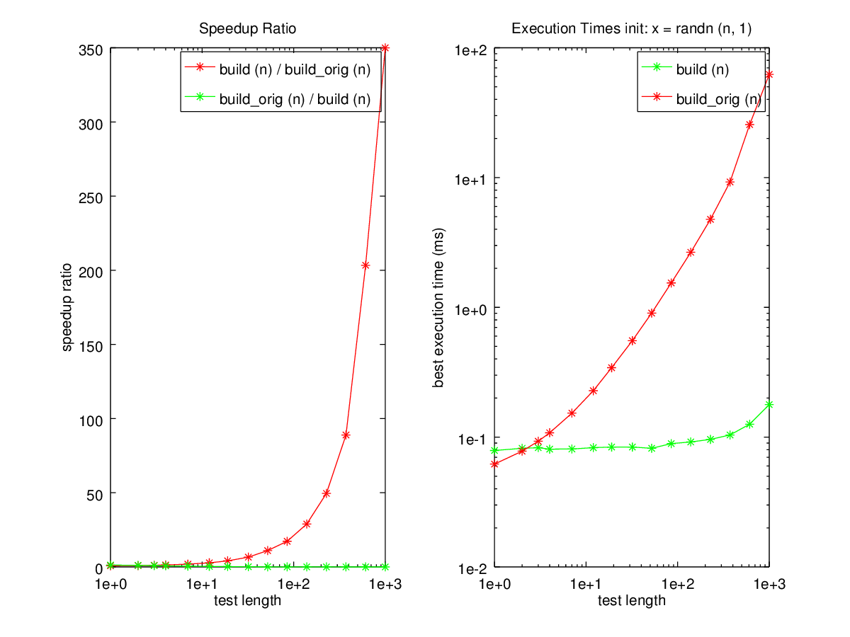
Produces the following output
-----------------------
function x = build_orig (n)
  for i=0:n-1, x([1:100]+i*100) = 1:100; endfor
endfunction
-----------------------
function x = build (n)
  idx = [1:100]';
  x = idx(:,ones(1,n));
  x = reshape (x, 1, n*100);
endfunction
-----------------------
Vectorized test.
This takes a little while...
testing build (n)
init: x = randn (n, 1)
n1 = 1  n2 = 2  n3 = 3  n4 = 4  n5 = 7  n6 = 12  n7 = 19  n8 = 32  n9 = 52  n10 = 85  n11 = 139  n12 = 228  n13 = 373  n14 = 611  n15 = 1000

Mean runtime ratio = 51.2 for 'build_orig (n)' vs 'build (n)'

For build (n):
  asymptotic power: O(n^0.2)
  approximate time per operation: 30 us
-----------------------
This time, the for loop is done away with entirely.
Notice how much bigger the speedup is than in example 1.
and the following figures
| Figure 1 | Figure 2 |
|---|---|
 |
 |
Package: octave