1 Getting Started 
This chapter takes you by the hand and gives a quick overview on the interval packages basic capabilities. More detailed information can usually be found in the functions’ documentation.
- Installation
- Set-based Interval Arithmetic
- Input and Output
- Arithmetic Operations
- Numerical Operations
- Boolean Operations
- Matrix and Array Operations
- Plotting
1.1 Installation 
It is recommended to install the package from specialized distributors for the particular platform, e. g., Debian GNU/Linux, MacPorts (for Mac OS X), FreshPorts (for FreeBSD), and so on. Since Octave version 4.0.1 the package is included in the official installer for Microsoft Windows and is installed automatically on that platform.
In any case, the interval package can alternatively be installed with the pkg command from within Octave. Latest release versions are published at Octave Forge and can be automatically downloaded with the -forge option.
pkg install -forge interval
  -| For information about changes from previous versions
  -| of the interval package, run 'news interval'.
During this kind of installation parts of the interval package are compiled for the target system, which requires development libraries for GNU Octave (version ≥ 4.2.0) and GNU MPFR (version ≥ 3.1.0) to be installed. It might be necessary to install packages “liboctave-dev” and “libmpfr-dev”, which are provided by most GNU distributions (names may vary).
In order to use the interval package during an Octave session, it must have been loaded, i. e., added to the path. In the following parts of the manual it is assumed that the package has been loaded, which can be accomplished with the pkg load interval command. It is recommended to add this command at the beginning of script files, especially if script files are published or shared. Automatic loading of the interval package can be activated by adding the line pkg load interval to your .octaverc file located in your user folder, for more information see Startup Files in GNU Octave manual.
That’s it. The package is ready to be used within Octave.
1.2 Set-based Interval Arithmetic 
The most important and fundamental concepts in the context of the interval package are:
- Intervals are closed, connected subsets of the real numbers. Intervals may be unbound (in either or both directions) or empty. In special cases
+infand-infare used to denote boundaries of unbound intervals, but any member of the interval is a finite real number. - Classical functions are extended to interval functions as follows: The result of function f evaluated on interval x is an interval enclosure of all possible values of f over x where the function is defined. Most interval arithmetic functions in this package manage to produce a very accurate such enclosure.
- The result of an interval arithmetic function is an interval in general. It might happen, that the mathematical range of a function consist of several intervals, but their union will be returned, e. g., 1 / [-1, 1] = [Entire].
More details can be found in Introduction to Interval Arithmetic.
1.3 Input and Output 
Before exercising interval arithmetic, interval objects must be created from non-interval data. There are interval constants empty and entire and the interval constructors @infsupdec/infsupdec (create an interval from boundaries), midrad (create an interval from midpoint and radius) and hull (create an interval enclosure for a list of mixed arguments: numbers, intervals or interval literals). The constructors are very sophisticated and can be used with several kinds of parameters: Interval boundaries can be given by numeric values or string values with decimal numbers.
Create intervals for performing interval arithmetic
## Interval with a single number
infsupdec (1)
  ⇒ ans = [1]_com
## Interval defined by lower and upper bound
infsupdec (1, 2)
  ⇒ ans = [1, 2]_com
## Boundaries are converted from strings
infsupdec ("3", "4")
  ⇒ ans = [3, 4]_com
## Decimal number
infsupdec ("1.1")
  ⇒ ans ⊂ [1.0999, 1.1001]_com
## Decimal number with scientific notation
infsupdec ("5.8e-17")
  ⇒ ans ⊂ [5.7999e-17, 5.8001e-17]_com
## Interval around 12 with uncertainty of 3
midrad (12, 3)
  ⇒ ans = [9, 15]_com
## Again with decimal numbers
midrad ("4.2", "1e-3")
  ⇒ ans ⊂ [4.1989, 4.2011]_com
## Interval members with arbitrary order
hull (3, 42, "19.3", "-2.3")
  ⇒ ans ⊂ [-2.3001, +42]_com
## Symbolic numbers
hull ("pi", "e")
  ⇒ ans ⊂ [2.7182, 3.1416]_com
Warning: In above examples decimal fractions are passed as a string to the constructor. Otherwise it is possible, that GNU Octave introduces conversion errors when the numeric literal is converted into a floating-point number before it is passed to the constructor. The interval construction is a critical process, but after this the interval package takes care of any further conversion errors, representational errors, round-off errors and inaccurate numeric functions.
Beware of the conversion pitfall
## The numeric constant 0.3 is an approximation of the
## decimal number 0.3.  An interval around this approximation
## will not contain the decimal number 0.3.
sprintf("%[.17g]", infsupdec (0.3))
  ⇒ ans = [0.29999999999999998, 0.29999999999999999]_com
## However, passing the decimal number 0.3 as a string
## to the interval constructor will create an interval which
## actually encloses the decimal number.
format short
infsupdec ("0.3")
  ⇒ ans ⊂ [0.29999, 0.30001]_com
For maximum portability it is recommended to use interval literals, which are standardized by IEEE Std 1788-2015. Both interval boundaries are then given as a string in the form [l, u]. The output in the examples above gives examples of several interval literals.
## Interval literal
infsupdec ("[20, 4.2e10]")
  ⇒ ans = [20, 4.2e+10]_com
The default text representation of intervals is not guaranteed to be exact, because this would massively spam console output. For example, the exact text representation of realmin would be over 700 decimal places long! However, the output is correct as it guarantees to contain the actual boundaries: a displayed lower (upper) boundary is always less (greater) than or equal to the actual boundary.
1.3.1 Interval Vectors, Matrices and Arrays 
Vectors, matrices and arrays of intervals can be created by passing numerical arrays, string or cell arrays to the interval constructors. With cell arrays it is also possible to mix several types of boundaries.
Interval arrays behave like normal arrays in GNU Octave and can be used for broadcasting and vectorized function evaluation. Vectorized function evaluation usually is the key to create very fast programs.
Create interval arrays
M = infsupdec (magic (3))
  ⇒ M = 3×3 interval matrix

    [8]_com   [1]_com   [6]_com
    [3]_com   [5]_com   [7]_com
    [4]_com   [9]_com   [2]_com
infsupdec (magic (3), magic (3) + 1)
  ⇒ ans = 3×3 interval matrix

    [8, 9]_com    [1, 2]_com   [6, 7]_com
    [3, 4]_com    [5, 6]_com   [7, 8]_com
    [4, 5]_com   [9, 10]_com   [2, 3]_com
infsupdec ("0.1; 0.2; 0.3; 0.4; 0.5")
  ⇒ ans ⊂ 5×1 interval vector

    [0.099999, 0.10001]_com
     [0.19999, 0.20001]_com
     [0.29999, 0.30001]_com
     [0.39999, 0.40001]_com
                  [0.5]_com
infsupdec ("1 [2, 3]; 4, 5, 6")
  ⇒ ans = 2×3 interval matrix

    [1]_com   [2, 3]_com   [Empty]_trv
    [4]_com      [5]_com       [6]_com
infsupdec ({1; eps; "4/7"; "pi"}, {2; 1; "e"; "0xff"})
  ⇒ ans ⊂ 4×1 interval vector

              [1, 2]_com
     [2.2204e-16, 1]_com
   [0.57142, 2.7183]_com
       [3.1415, 255]_com
infsupdec (ones (2, 2, 2))
  ⇒ ans = 2×2×2 interval array

  ans(:,:,1) =

     [1]_com   [1]_com
     [1]_com   [1]_com

  ans(:,:,2) =

     [1]_com   [1]_com
     [1]_com   [1]_com
Strings can easily be used to create vectors and matrices of intervals, , and ; are used to denote the next element in the row or a new row. Octave does however not have way of representing arrays with three or more dimensions using strings in the same way. Therefore you can only create such arrays by passing numerical matrices or cells to the constructor. Alternatively you can build it up in steps.
A = infsupdec ("1 [2, 3]; 4, 5; 6, 7")
  ⇒ A = 3×2 interval matrix

     [1]_com   [2, 3]_com
     [4]_com      [5]_com
     [6]_com      [7]_com

A(:,:,2) = infsupdec ("0.1, 0.2; 0.3, 0.4; 0.5, 0.6")
  ⇒ A ⊂ 3×2×2 interval array

  ans(:,:,1) =

     [1]_com   [2, 3]_com
     [4]_com      [5]_com
     [6]_com      [7]_com

  ans(:,:,2) =

     [0.099999, 0.10001]_com   [0.19999, 0.20001]_com
      [0.29999, 0.30001]_com   [0.39999, 0.40001]_com
                   [0.5]_com   [0.59999, 0.60001]_com
1.4 Arithmetic Operations 
The interval package comprises many interval arithmetic operations. A complete list can be found in its function reference. Function names match GNU Octave standard functions where applicable and follow recommendations by IEEE Std 1788-2015 otherwise, see Function Names.
The interval arithmetic flavor used by this package is the “set-based” interval arithmetic and follows these rules: Intervals are sets. They are subsets of the set of real numbers. The interval version of an elementary function such as sin(x) is essentially the natural extension to sets of the corresponding point-wise function on real numbers. That is, the function is evaluated for each number in the interval where the function is defined and the result must be an enclosure of all possible values that may occur.
By default arithmetic functions are computed with best possible accuracy (which is more than what is guaranteed by GNU Octave core functions). The result will therefore be a tight and very accurate enclosure of the true mathematical value in most cases. Details on each function’s accuracy can be found in its documentation, which is accessible with GNU Octave’s help command.
Examples of using interval arithmetic functions
sin (infsupdec (0.5))
  ⇒ ans ⊂ [0.47942, 0.47943]_com
power (infsupdec (2), infsupdec (3, 4))
  ⇒ ans = [8, 16]_com
atan2 (infsupdec (1), infsupdec (1))
  ⇒ ans ⊂ [0.78539, 0.7854]_com
midrad (magic (3), 0.5) * pascal (3)
  ⇒ ans = 3×3 interval matrix

    [13.5, 16.5]_com   [25, 31]_com   [42, 52]_com
    [13.5, 16.5]_com   [31, 37]_com   [55, 65]_com
    [13.5, 16.5]_com   [25, 31]_com   [38, 48]_com
1.5 Numerical Operations 
Some interval functions do not return an interval enclosure, but a single number (in binary64 precision). Most important are @infsup/inf and @infsup/sup, which return the lower and upper interval boundaries.
More such operations are @infsup/mid (approximation of the interval’s midpoint), @infsup/wid (approximation of the interval’s width), @infsup/rad (approximation of the interval’s radius), @infsup/mag (interval’s magnitude) and @infsup/mig (interval’s mignitude).
## Enclosure of the decimal number 0.1 is not exact
## and results in an interval with a small uncertainty.
wid (infsupdec ("0.1"))
  ⇒ ans =    1.3878e-17
1.6 Boolean Operations 
Interval comparison operations produce boolean results. While some comparisons are especially for intervals (@infsup/subset, @infsup/interior, @infsup/ismember, @infsup/isempty, @infsup/disjoint, …) others are interval extensions of simple numerical comparison. For example, the less-or-equal comparison is mathematically defined as ∀a ∃b a ≤ b ∧ ∀b ∃a a ≤ b.
infsup (1, 3) <= infsup (2, 4)
  ⇒ ans = 1
1.7 Matrix and Array Operations 
Above mentioned operations can also be applied element-wise to interval vectors, matrices or arrays. Many operations use vectorization techniques.
In addition, there are operations on interval matrices and arrays. These operations comprise: dot product, matrix multiplication, vector sums (all with tightest accuracy), matrix inversion, matrix powers, and solving linear systems (the latter are less accurate). As a result of missing hardware / low-level library support and missing optimizations, these operations are relatively slow compared to familiar operations in floating-point arithmetic.
Examples of using interval matrix functions
A = infsupdec ([1, 2, 3; 4, 0, 0; 0, 0, 1]);
A (2, 3) = "[0, 6]"
  ⇒ A = 3×3 interval matrix

    [1]_com   [2]_com      [3]_com
    [4]_com   [0]_com   [0, 6]_com
    [0]_com   [0]_com      [1]_com
B = inv (A)
  ⇒ B = 3×3 interval matrix

      [0]_trv     [0.25]_trv       [-1.5, 0]_trv
    [0.5]_trv   [-0.125]_trv   [-1.5, -0.75]_trv
      [0]_trv        [0]_trv             [1]_trv
A * B
  ⇒ ans = 3×3 interval matrix

    [1]_trv   [0]_trv   [-1.5, +1.5]_trv
    [0]_trv   [1]_trv       [-6, +6]_trv
    [0]_trv   [0]_trv            [1]_trv
A = infsupdec (magic (3))
  ⇒ A = 3×3 interval matrix

    [8]_com   [1]_com   [6]_com
    [3]_com   [5]_com   [7]_com
    [4]_com   [9]_com   [2]_com
c = A \ [3; 4; 5]
  ⇒ c ⊂ 3×1 interval vector

    [0.18333, 0.18334]_trv
    [0.43333, 0.43334]_trv
    [0.18333, 0.18334]_trv
A * c
  ⇒ ans ⊂ 3×1 interval vector

    [2.9999, 3.0001]_trv
    [3.9999, 4.0001]_trv
    [4.9999, 5.0001]_trv
1.7.1 Notes on Linear Systems 
A system of linear equations in the form Ax = b with intervals can be seen as a range of classical linear systems, which can be solved simultaneously. Whereas classical algorithms compute an approximation for a single solution of a single linear system, interval algorithms compute an enclosure for all possible solutions of (possibly several) linear systems. Some characteristics should definitely be known when linear interval systems are solved:
- If the linear system is underdetermined and has infinitely many solutions, the interval solution will be unbound in at least one of its coordinates. Contrariwise, from an unbound result it can not be concluded whether the linear system is underdetermined or has solutions.
- If the interval result is empty in at least one of its coordinates, the linear system is guaranteed to be overdetermined and has no solutions. Contrariwise, from a non-empty result it can not be concluded whether all or some of the systems have solutions or not.
- Wide intervals within the matrix A can easily lead to a superposition of cases, where the rank of A is no longer unique. If the linear interval system contains cases of linear independent equations as well as linear dependent equations, the resulting enclosure of solutions will inevitably be very broad.
However, solving linear systems with interval arithmetic can produce useful results in many cases and automatically carries a guarantee for error boundaries. Additionally, it can give better information than the floating-point variants for some cases.
Standard floating point arithmetic versus interval arithmetic on ill-conditioned linear systems
A = [1, 0; 2, 0];
## This linear system has no solutions
A \ [3; 0]
  -| warning: ...matrix singular to machine precision...
  ⇒ ans =

       0.6000
            0
## This linear system has many solutions
A \ [4; 8]
  ⇒ ans =

       4
       0
## The empty interval vector proves that there is no solution
infsup (A) \ [3; 0]
  ⇒ ans = 2×1 interval vector

       [Empty]
       [Empty]
## The unbound interval vector indicates
## that there may be many solutions
infsup (A) \ [4; 8]
  ⇒ ans = 2×1 interval vector

            [4]
       [Entire]
1.8 Plotting 
Plotting of intervals in 2D and 3D can be achieved with the functions @infsup/plot and @infsup/plot3 respectively. However, some differences in comparison with classical plotting in Octave shall be noted.
When plotting classical (non-interval) functions in Octave, one normally uses a vector and evaluates a function on that vector element-wise. The resulting X and Y (and possibly Z) coordinates are then drawn against each other, whilst coordinates can be connected using interpolated lines. The plot shows an approximation of the function’s graph and the accuracy (and smoothness of the graph) primarily depends on the number of coordinates where the function has been evaluated.
Evaluating the same function on a single interval (e. g. the part of the function’s domain that is of interest) yields a single interval result which covers the actual range of the function. Plotting just two intervals, input and output, against each other is boring, because the plot would only show a single rectangle. Contrariwise, evaluating the function for many individual points (e. g. using @infsup/linspace) would hardly fit in the philosophy of interval arithmetic. Individual points of evaluation are not interconnected by the interval plotting functions, because that would introduce errors.
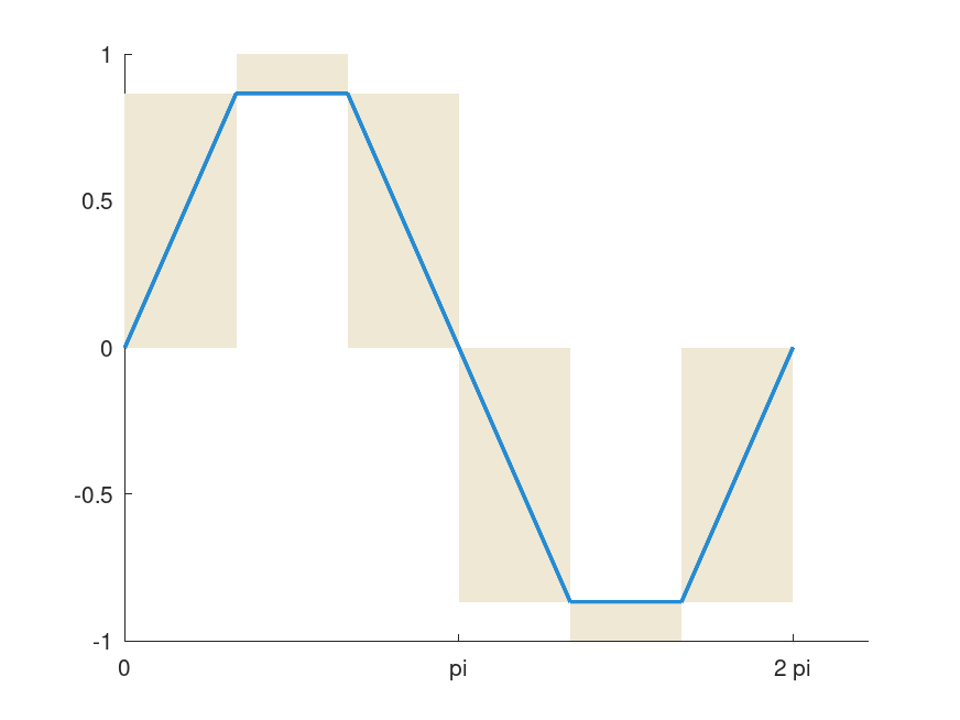
The solution for plotting functions with interval arithmetic is called: “mincing”. The @infsup/mince function divides an interval into many smaller adjacent subsets, which can be used for range evaluations of the function. As a result, one gets vectors of intervals, which produce a coverage of the function’s graph using rectangles. Please note, how the rectangles cover the sine function’s true range from −1 to 1 in the following example, whilst the interpolated lines make a poor approximation.
hold on
blue = [38 139 210] ./ 255;
shade = [238 232 213] ./ 255;
## Interval plotting
x = mince (2*infsup (0, "pi"), 6);
plot (x, sin (x), shade)
## Classical plotting
x = linspace (0, 2*pi, 7);
plot (x, sin (x), 'linewidth', 2, 'color', blue)
set (gca, 'XTick', 0 : pi : 2*pi)
set (gca, 'XTickLabel', {'0', 'pi', '2 pi'})
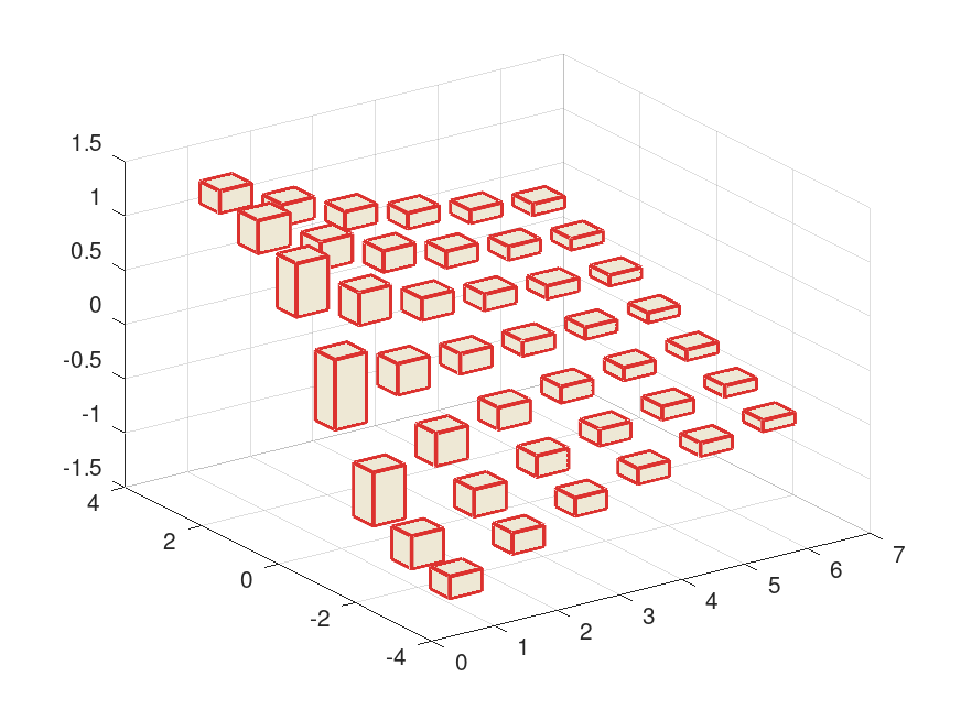
For 3D plotting the Octave meshgrid function, as usual, becomes handy. The following example shows how two different ranges for X and Y coordinates are used to construct a grid, where the function @infsup/atan2 is evaluated. In this particular case the interval grid has gaps, because X and Y coordinates have been constructed such that intervals do not intersect.
red = [220 50 47] ./ 255;
shade = [238 232 213] ./ 255;
x = midrad (1 : 6, 0.25);
y = midrad (-3 : 3, 0.25);
[x, y] = meshgrid (x, y);
z = atan2 (y, x);
plot3 (x, y, z, shade, red)
view ([-35, 30])
box off
set (gca, "xgrid", "on", "ygrid", "on", "zgrid", "on")